💡 Direct Answer & Executive Summary (Bacterial Growth Logarithmic Phase Solver)
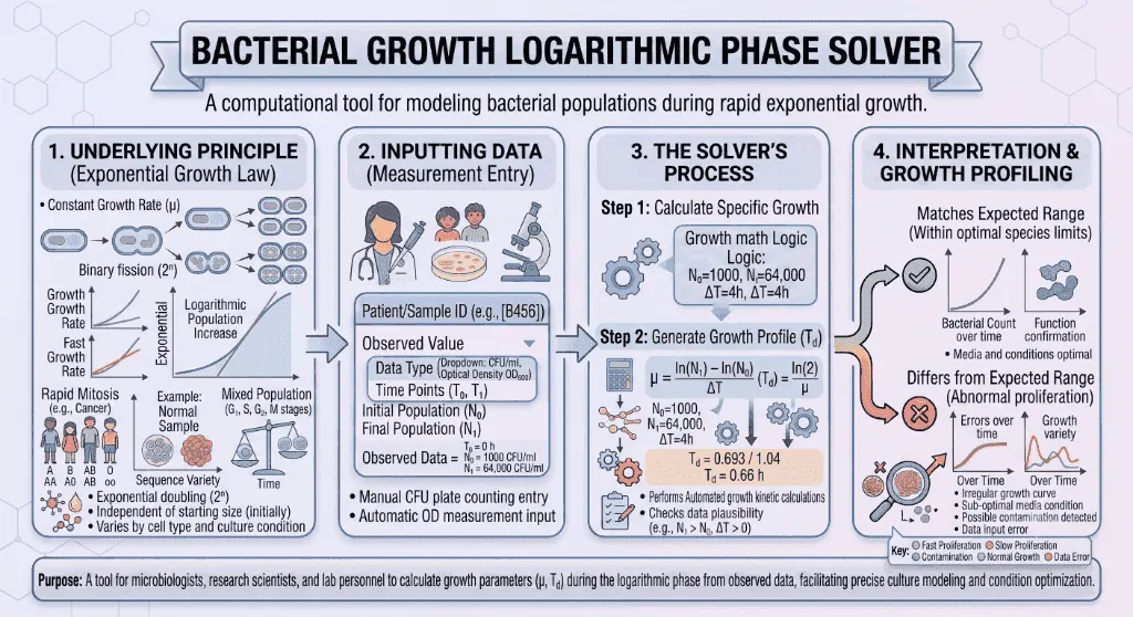
Definition: Calculate bacterial exponential growth kinetics, specific growth rate (μ), generation time (g / Td), total generations (n), and final population (Nt) during logarithmic phase.
Governing Math Formula: Binary Fission: Nt = N0 × 2^n. Specific Growth Rate: μ = [ln(Nt) - ln(N0)] / Δt. Generation Time: g = ln(2) / μ = 0.69315 / μ. Total Generations: n = 3.3219 × log10(Nt / N0).
Target Applications: Provides real-time quantitative solutions in Biology for students, engineers, researchers, and finance professionals.
Bacterial Growth Logarithmic Phase Solver: Binary Fission, Specific Growth Rate & Generation Time Guide
1. Introduction
In microbiology, industrial fermentation, clinical diagnostics, and food safety, understanding how bacterial populations multiply is fundamental to predicting outbreaks, harvesting biopharmaceuticals, and formulating antibiotic regimens.
Bacterial reproduction occurs via binary fission, a process of asexual cellular division where a single vegetative parent cell duplicates its genomic material, elongates, and cleaves into two genetically identical daughter cells. Under optimal physiological conditions with abundant nutrients and unconstrained space, this process drives an explosive, geometric population expansion termed the Logarithmic (Exponential) Growth Phase.
During the logarithmic phase, the population doubles at a constant, species-specific tempo. A minute contamination of in unpasteurized dairy or industrial broth can surge to over within just four hours, rapidly breaching international food safety thresholds or reaching peak cell density for recombinant protein induction.
How do microbiologists calculate the specific growth rate () and generation time ()? What mathematical formulas govern binary fission? How does optical density () translate into viable colony-forming units ()?
This comprehensive guide details the mathematical equations, microbial mechanics, growth curve phases, and industrial case studies governing bacterial logarithmic growth.
flowchart LR
    INOC["🧫 Bacterial Inoculum
Initial Population (N0)
Plate Count / OD600 Turbidity"] --> BINARY["⚡ Binary Fission (2ⁿ)
FtsZ Divisome Septum Cleavage
Logarithmic Exponential Phase"]
    BINARY --> SOLVER["🧮 Log Growth Kinetic Solver
Specific Growth Rate (μ)
Generation / Doubling Time (g)"]
    SOLVER --> IMPACT["🏭 Real-World Action
Food Safety HACCP, Fermentation Titer & MIC Kill Curves"]
2. Definitions
2.1 Simple Everyday Definition
The Logarithmic Phase (or Exponential Phase) is the period when bacteria multiply at their fastest possible rate, with the population continuously doubling at fixed time intervals (like ).
2.2 Formal Technical Definition
The Logarithmic Growth Phase is the physiological state of a closed microbial culture where cells are in balanced growth, synthesizing cellular components at identical relative rates, such that the population increases in proportion to its instantaneous size:
Where:
- is the Initial Population at time ( or total cell count).
- is the Final Population at time ().
- is the Specific Growth Rate (, typically ).
- is the Number of Completed Generations (doublings).
- $\Delta t$ is the Elapsed Incubation Duration ().
- Generation Time ( or ): The time interval required for the bacterial population to double in number:
2.3 Vivid Real-World Analogies
The Doubling Grain of Rice on the Chessboard:
Place grain of rice on the first square of a chessboard, on the second, on the third, on the fourth, and on the fifth. By the square, the total exceeds . Bacterial binary fission behaves identically: a single bacterium with a doubling time produces over in just .
The Self-Replicating Factory:
Imagine a machine in an industrial plant that spends building an exact working duplicate of itself. After , you have factories; after , factories; after , factories. Each new machine immediately starts building another machine at the exact same velocity.
3. History & Scientific Milestones
The mathematical characterization of bacterial growth transformed microbiology from descriptive natural history into a quantitative predictive science.
flowchart TD
    H1["📅 1881: Robert Koch
Develops solid agar media, enabling pure culture isolation & CFU colony counts"] --> H2["📅 1942: Jacques Monod
Formulates bacterial growth mathematics & Monod kinetics (Nobel Prize 1965)"]
    H2 --> H3["📅 1949: Arthur Finch Ellis
Standardizes turbidimetric spectrophotometry for optical density (OD600)"]
    H3 --> H4["📅 1958: Maaløe & Kjeldgaard (Copenhagen School)
Defines balanced exponential growth and macromolecular ribosomal scaling"]
    H4 --> H5["📅 1969: Thomas Brock
Discovers Thermus aquaticus in Yellowstone; defines extremophile doubling limits"]- Robert Koch & Julius Petri (1881–1887): Developed solid agar nutrient plates and Petri dishes, establishing the Colony-Forming Unit () method to quantify viable bacterial populations.
- Jacques Monod (1942): Published Recherches sur la croissance des cultures bactériennes, deriving the mathematical equations for specific growth rate and the Monod Equation, which relates bacterial growth velocity to substrate concentration.
- Ole Maaløe & Niels Ole Kjeldgaard (1958): Established the "Copenhagen School" of bacterial physiology, proving that during balanced exponential growth, bacterial mass, RNA content, and protein synthesis scale in exact geometric harmony.
- Thomas Brock (1969): Isolated Thermus aquaticus from boiling hot springs in Yellowstone National Park, proving that bacterial binary fission kinetics operate even at and providing the heat-stable Taq polymerase that enabled the Polymerase Chain Reaction (PCR).
4. Core Concepts & Biochemical Mechanisms
graph TD
    CURVE["📈 The 4 Classical Phases of Microbial Batch Culture"]

    CURVE --> LAG["1. Lag Phase
• Zero net population increase
• Intense metabolic adaptation & enzyme synthesis
• Ribosome & ATP accumulation"]
    CURVE --> LOG["2. Log / Exponential Phase
• Balanced binary fission (2ⁿ)
• Constant maximal growth rate (μ = μ_max)
• Population doubles at fixed generation time (g)"]
    CURVE --> STAT["3. Stationary Phase
• Nutrients depleted; toxic metabolic wastes accumulate
• Growth rate equals death rate (μ = d)
• Endospore formation & secondary metabolites"]
    CURVE --> DEATH["4. Death / Decline Phase
• Exponential loss of viable cells (CFU drop)
• Lysis & nutrient scavenging"]
4.1 The Four Phases of Bacterial Growth
- Lag Phase: Inoculated bacteria adjust to their new environment. Cells synthesize necessary metabolic enzymes, RNA, and structural proteins. No net change in cell number occurs.
- Logarithmic (Exponential) Phase: Cells divide at the maximum rate possible for the given medium, temperature, and aeration. Population growth follows strict geometric scaling.
- Stationary Phase: Essential nutrients (carbon, nitrogen, oxygen) become depleted, and inhibitory metabolic byproducts (lactic acid, acetate, ethanol) accumulate. The rate of cell division equals the rate of cell death ().
- Death Phase: Toxic waste concentrations overwhelm cellular defense mechanisms, and viable cell counts drop exponentially.
4.2 Molecular Machinery of Binary Fission
- The FtsZ Ring (Divisome): The tubulin-like GTPase protein FtsZ polymerizes into a contractile ring at the mid-cell division plane.
- Peptidoglycan Synthesis: Autolysins create controlled nicks in the existing cell wall, while Penicillin-Binding Proteins () cross-link newly synthesized and disaccharide subunits into the growing septum.
- Chromosome Segregation: The circular bacterial chromosome undergoes bidirectional theta () replication from the origin (oriC) to the terminus (ter), with the two daughter chromosomes tethered to opposite poles of the plasma membrane prior to septation.
5. Formulas & Mathematical Derivations
5.1 Exponential Growth Law (Binary Fission)
Taking the base-10 logarithm () of both sides:
5.2 Specific Growth Rate ()
In continuous exponential terms:
5.3 Generation Time ( or )
When the population doubles (), the elapsed time $\Delta t$ equals the generation time :
5.4 Monod Substrate Growth Kinetics
When growth is limited by an essential nutrient substrate concentration $[S]$:
Where is the maximum achievable growth rate and is the half-velocity substrate affinity constant.
5.5 Variable Reference Table
| Parameter | Symbol | Standard Units | Biological Role |
|---|---|---|---|
| Initial Population | or total cells | Inoculum density at the start of log phase | |
| Final Population | or total cells | Population density at time | |
| Elapsed Time | $\Delta t$ | Hours () | Duration of incubation during exponential phase |
| Generations | Dimensionless count | Number of binary fission population doublings | |
| Specific Growth Rate | Instantaneous velocity of biomass accumulation | ||
| Generation Time | () | Minutes or Hours | Time required for population to double |
| Optical Density | Absorbance Units () | Turbidimetric light scattering index at |
6. Step-by-Step Computational Walkthrough
Let us calculate the growth parameters for an unpasteurized milk contamination scenario:
- Initial contamination: ()
- Final count: ()
- Incubation time at room temperature ():
flowchart TD
    STEP1["Step 1: Calculate Population Fold Expansion
Fold = Nt / N0 = 64,000 / 1,000 = 64.0×"] --> STEP2["Step 2: Solve Number of Completed Generations (n)
n = log2(64) = 6.0 Completed Generations"]
    STEP2 --> STEP3["Step 3: Calculate Specific Growth Rate (μ)
μ = ln(64) / 4.0 h = 4.15888 / 4.0 = 1.0397 h⁻¹"]
    STEP3 --> STEP4["Step 4: Solve Generation / Doubling Time (g)
g = 0.69315 / 1.0397 = 0.6667 Hours = 40.0 Minutes"]
    STEP4 --> STEP5["Step 5: Compare Against Food Safety Thresholds
64,000 CFU/mL exceeds Grade A milk standard (<20,000 CFU/mL)"]- Step 1: Calculate Fold Expansion:
- Step 2: Solve Number of Generations ():
- Step 3: Calculate Specific Growth Rate ():
- Step 4: Solve Generation Time ():
- Step 5: Biological Evaluation:A generation time of is characteristic of mesophilic foodborne pathogens (such as Salmonella enterica or Listeria monocytogenes) rapidly multiplying at ambient temperature.
7. Visual Explanations & Growth Curve Dynamics
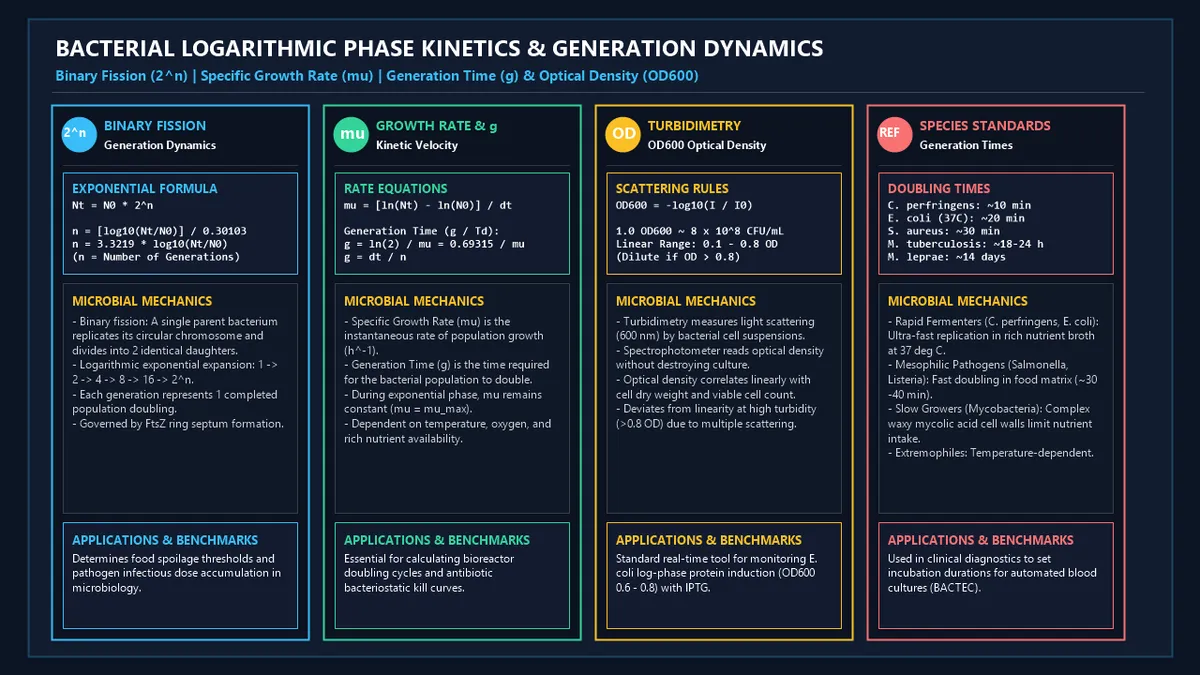
flowchart TD
    SPECTRUM["Microbial Generation Time (g) Spectrum Across Bacteria"]

    SPECTRUM --> ULTRA["🚀 Hyper-Fast Replicators (g: 10 - 20 min)
• Clostridium perfringens (g ≈ 10 min)
• Vibrio cholerae (g ≈ 11 - 13 min)
• Escherichia coli BL21 at 37°C (g ≈ 20 min)"]
    SPECTRUM --> MESO["🌿 Standard Mesophilic Pathogens (g: 25 - 60 min)
• Staphylococcus aureus (g ≈ 30 min)
• Salmonella enterica (g ≈ 35 - 40 min)
• Listeria monocytogenes (g ≈ 45 min)"]
    SPECTRUM --> MOD["🐢 Moderate Environmental Bacteria (g: 1 - 3 hours)
• Bacillus subtilis (g ≈ 60 min)
• Pseudomonas putida (g ≈ 90 min)
• Rhizobium leguminosarum (g ≈ 120 min)"]
    SPECTRUM --> SLOW["⏳ Slow-Growing Acid-Fast & Oligotrophs (g > 12 hours)
• Mycobacterium tuberculosis (g ≈ 18 - 24 hours)
• Treponema pallidum (g ≈ 30 - 33 hours)
• Mycobacterium leprae (g ≈ 14 days)"]
8. Comparative & Standards Tables
8.1 Generation Times & Specific Growth Rates Across Bacterial Species ()
| Bacterial Species | Gram Stain & Morphology | Optimum Temp | Generation Time () | Specific Growth Rate () | Biological Significance |
|---|---|---|---|---|---|
| Clostridium perfringens | Gram-positive bacillus | Fastest recorded bacterial doubler; gas gangrene | |||
| ***Escherichia coli* (K-12/B)** | Gram-negative bacillus | Laboratory model & recombinant expression host | |||
| Vibrio cholerae | Gram-negative curved rod | Rapid diarrheal hyper-proliferation in gut lumen | |||
| Staphylococcus aureus | Gram-positive coccus | Skin abscesses, MRSA bacteremia, enterotoxin | |||
| Salmonella enterica | Gram-negative bacillus | Foodborne gastroenteritis & enteric fever | |||
| Listeria monocytogenes | Gram-positive bacillus | Psychrotolerant food pathogen (grows at ) | |||
| Pseudomonas aeruginosa | Gram-negative bacillus | Opportunistic biofilm pathogen in cystic fibrosis | |||
| Mycobacterium tuberculosis | Acid-fast bacillus | Waxy mycolic acid cell wall slows nutrient flux | |||
| Mycobacterium leprae | Acid-fast bacillus | Slowest known pathogen; causative agent of leprosy |
8.2 Optical Density () vs. Viable Cell Density Calibration (E. coli)
| Optical Density () | Physical Appearance | Approximate Cell Count () | Growth Phase State | Recommended Action |
|---|---|---|---|---|
| Faint hazy broth | Early Log Phase | Inoculum confirmation | ||
| Noticeably turbid | Mid-Log Phase | Preparation of electrocompetent cells | ||
| Milky opaque broth | Late-Log Phase | Optimal IPTG induction of recombinant proteins | ||
| Dense opaque broth | Early Stationary Phase | Cell harvesting for plasmid extraction | ||
| Heavy suspension | Deep Stationary Phase | Dilute sample $1:10$ for accurate spectrophotometry |
9. Practical Real-World Applications
Example 1: Food Safety HACCP Critical Temperature Limits
Federal food safety standards mandate that perishable foods must not remain in the "Danger Zone" () for more than . Calculating specific growth rates demonstrates that Salmonella counts increase over () every at room temperature.
Example 2: Industrial Bioreactor Recombinant Protein Induction
In biopharmaceutical manufacturing of human insulin, growth kinetics dictate the exact timing of chemical inducer addition (). Inducing at (Late-Log Phase) maximizes protein expression while maintaining high cellular ribosomal capacity.
Example 3: Automated Blood Culture Detection in Sepsis (BACTEC)
Automated clinical blood culture systems continuously monitor fluorescent sensor signals. By calculating the slope of logarithmic production, the instrument alerts microbiologists to positive bacteremia within of incubation.
10. In-Depth Case Studies
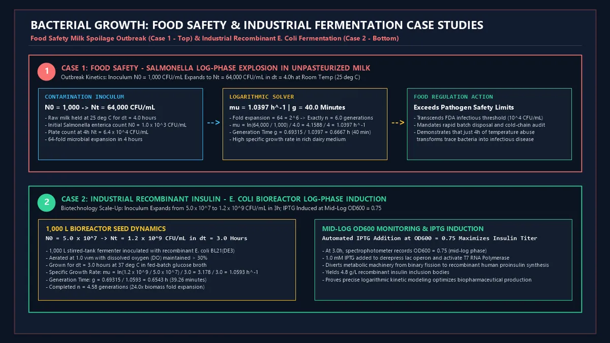
Case Study 1: Food Safety — Salmonella Log-Phase Explosion in Unpasteurized Milk
- Outbreak Investigation: An artisanal dairy farm experiences a refrigeration compressor failure. Raw milk sits at room temperature () for .
- Laboratory Microbiological Testing:- Initial Salmonella enterica contamination:- Quantitative plate count at :
- Kinetic Calculations:
- Regulatory Action: The final bacterial density () breached the Grade A pasteurized milk regulatory limit (). The entire batch was condemned and discarded, preventing an outbreak of salmonellosis.
Case Study 2: Industrial Recombinant Insulin — E. coli Bioreactor Log-Phase Induction
- Biotechnology Objective: Maximize recombinant human proinsulin inclusion body yield in a industrial stirred-tank fermenter using E. coli BL21(DE3).
- Seed Fermentation Tracking:- Inoculum density:- Density after of fed-batch glucose feeding at :
- Logarithmic Kinetic Profile:
- Optimization Strategy:- Spectrophotometer tracked optical density to (Mid-to-Late Log Phase) at .- was injected automatically, derepressing the lac operon and activating T7 RNA polymerase.- The culture yielded of recombinant insulin protein, confirming that induction during logarithmic growth maximizes recombinant productivity.
11. Advantages of Mathematical Bacterial Growth Modeling
- Predictive Food Safety & Shelf-Life Modeling: Accurately forecasts microbial load under fluctuating storage temperatures.
- Optimizes Industrial Fermentation Harvests: Pinpoints the exact physiological window for nutrient feeding and gene induction.
- Determines Antibiotic Pharmacodynamics: Measures bactericidal kill rates () and post-antibiotic effect () durations.
- Enables Real-Time Turbidimetric Monitoring: Correlates non-destructive optical density measurements with viable cell counts.
12. Methodological Complexities & Artifacts
- Non-Linear Optical Density Above : At high cell densities, light scattered by one bacterium is re-scattered by adjacent bacteria (multiple scattering), causing the spectrophotometer to underestimate true cell density. Samples must be diluted $1:5$ or $1:10$.
- Viable But Non-Culturable () State: Stressed pathogens (e.g., Vibrio, Campylobacter) remain metabolically active but fail to form visible colonies on standard agar plates, underestimating true viable populations.
- Clumping & Filamentation: Bacteria growing in clusters (Staphylococci) or chains (Streptococci) form a single colony from multiple cells, requiring vigorous vortexing before plating.
13. Common Mistakes to Avoid
1. Calculating Growth Rate Across the Lag or Stationary Phase:
The formulas and are mathematically valid only during the pure exponential log phase. Including lag or stationary time points artificially depresses .
2. Mixing Base-10 () and Natural Log ($\ln$):
When calculating specific growth rate , use natural log ($\ln$). When calculating generations with base-10 log, remember the conversion constant $3.3219$ ().
3. Measuring Absorbance Without Blanking:
Failing to blank the spectrophotometer with sterile uninoculated growth medium distorts optical density readings.
12. Frequently Asked Questions (FAQ)
What is the difference between specific growth rate () and generation time ()?
Specific growth rate () is the instantaneous speed of population growth (expressed in reciprocal hours, ). Generation time () is the actual time (in minutes or hours) required for the population to double ().
Why does bacterial growth slow down during the stationary phase?
Growth slows down because essential nutrients (carbon sources, trace minerals, dissolved oxygen) are exhausted, and toxic metabolic wastes (acids, alcohols, reactive oxygen species) accumulate in the closed culture vessel.
What optical density () corresponds to for E. coli?
For standard E. coli strains, an of corresponds to approximately .
Can bacteria grow exponentially forever in a continuous culture?
In a batch culture, no; resources run out. However, in a chemostat (continuous bioreactor), fresh sterile nutrient broth is continuously added while spent medium and cells are removed at an equal rate, maintaining bacteria in indefinite logarithmic growth.
Why is Mycobacterium tuberculosis so slow-growing compared to E. coli?
M. tuberculosis has a generation time of because its cell envelope is rich in dense, hydrophobic mycolic acids, which severely restrict the rate of nutrient and hydrophilic substrate transport into the cell.
How does temperature affect the logarithmic growth rate?
Within a species' permissive range, growth rate increases with temperature up to an optimum (roughly doubling every , ). Beyond the optimum, essential enzymes denature and membrane fluidity collapses, causing a sharp drop in growth.
How do you convert optical density to cell dry weight?
By constructing an empirical standard curve where known volumes of culture at various values are pelleted, washed, desiccated in an oven at , and weighed on an analytical balance.
15. Expert Tips for Microbiologists, Fermentation Engineers & Food Safety Specialists
- Dilute Samples When : Keep your spectrophotometer readings in the linear absorbance range () by diluting thick suspensions in sterile isotonic saline.
- Harvest Recombinant Proteins at Mid-to-Late Log Phase: Inject IPTG when hits to maximize cellular translation machinery before stationary phase proteases are expressed.
- Log-Transform Plate Counts for Linear Plotting: Plot versus time to produce a straight line whose slope () allows instant visual confirmation of exponential phase boundaries.
16. Summary Checklist
- ✔ Determine Initial () and Final () Cell Counts: Obtain viable CFU plate counts or calibrate absorbance.
- ✔ Verify Logarithmic Phase Integrity: Ensure measurements are taken within the linear exponential window.
- ✔ Calculate Number of Generations (): Solve .
- ✔ Compute Specific Growth Rate (): Solve .
- ✔ Determine Generation / Doubling Time (): Solve .
- ✔ Correlate with Physiological Standards: Classify growth velocity (Rapid Fermenter, Mesophile, Slow Mycobacteria).
- ✔ Apply to Quality & Process Control: Guide food safety cold chains or bioreactor IPTG induction schedules.
Additional Technical Guidelines & Measurement Standards
When conducting calculations for Bacterial Growth Logarithmic Phase Solver, maintaining quantitative precision and verifying input parameter boundaries is essential for reliable scenario evaluation. Always verify that raw numerical inputs are measured using standardized instrumentation, and double-check unit conversions prior to applying outputs in commercial, industrial, or academic projects.
For quantitative unit conversions and scientific calculations, always maintain at least four decimal places of precision during intermediate arithmetic stages before rounding final results. When preparing technical reports, laboratory documentation, or financial forecasts, cross-verify all output variables against established international measurement standards (such as SI, NIST, and ISO metric benchmarks) to guarantee consistent analytical rigor across all computational workflows.
MathsLover.com delivers this interactive solver 100% free of charge to foster global mathematical literacy, educational accessibility, and data-driven problem solving across scientific, technical, and academic communities worldwide.