Beer-Lambert Absorbance Spectroscopy ($A = \varepsilon \cdot c \cdot l$)

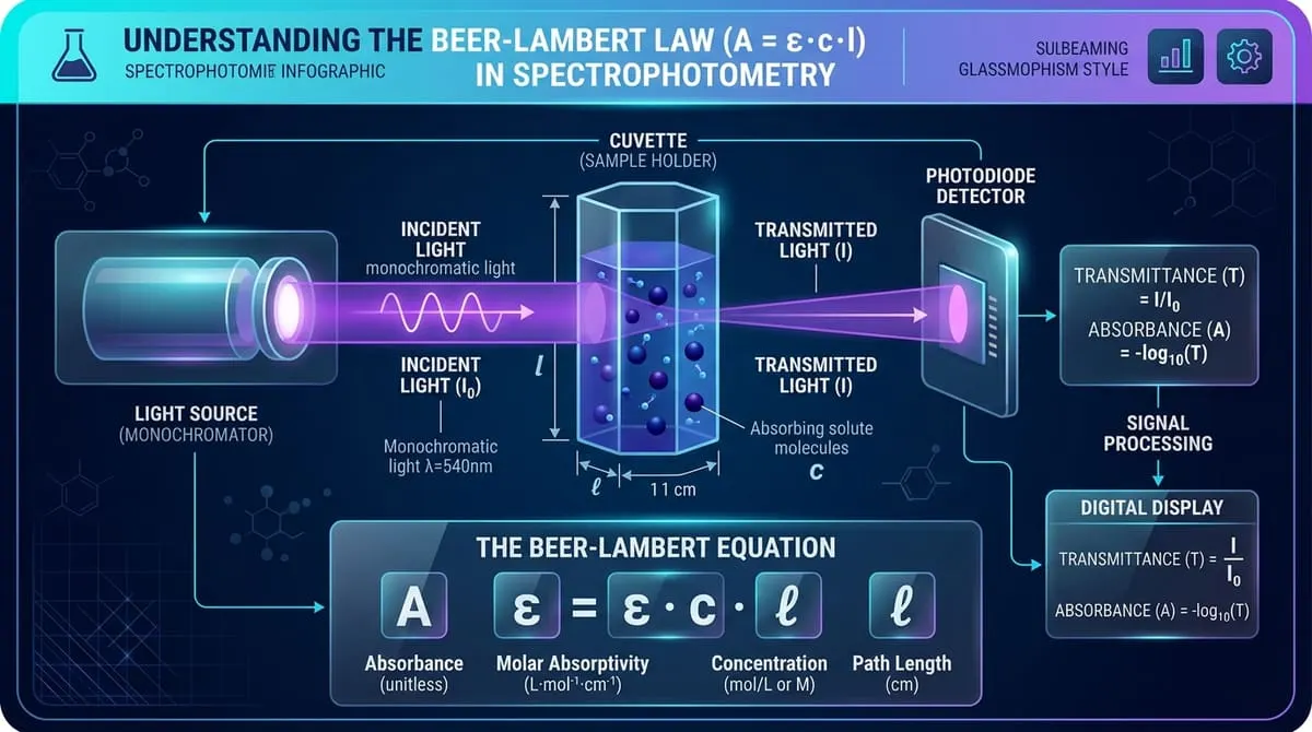
1. Introduction & Conceptual Overview

How do clinical laboratory analyzers measure the exact concentration of glucose, cholesterol, or therapeutic drugs in a single drop of human blood plasma? How do environmental monitoring stations detect parts-per-million toxic heavy metals in municipal drinking water? How do molecular biologists quantify pure DNA, RNA, and protein yields in nanodrop micro-spectrophotometers?

Every single one of these analytical, biochemical, and pharmaceutical measurements relies on the Beer-Lambert Law (also known as the Beer-Lambert-Bouguer Law or simply Beer's Law).

Formulated through the progressive optical discoveries of Pierre Bouguer (1729), Johann Heinrich Lambert (1760), and August Beer (1852), this foundational principle of optical spectroscopy establishes the direct, linear relationship between the optical absorbance ($A$) of a light-absorbing chemical substance and its molar concentration ($c$), molar absorptivity ($\varepsilon$), and the path length ($l$) of the light beam.

flowchart TD
    subgraph OPT["🔬 1. Spectrophotometer Optical Path"]
        L["💡 Light Source (Monochromator at λ_max)"]
        C["🧪 Sample Cuvette (Path Length: l = 1 cm, Concentration: c)"]
        D["⚡ Photodiode Detector (Measures Transmitted Intensity I)"]
        
        L -->|"Incident Light (I₀)"| C
        C -->|"Transmitted Light (I)"| D
    end
    
    subgraph OUT["📊 2. Spectroscopic Output Quantification"]
        A["Transmittance: T = I / I₀
Absorbance: A = -log₁₀(T) = ε × c × l"]
    end
    
    OPT --> OUT

2. Chemical Definition & Physical Theory

2.1 Simple Definition (Everyday Language)

In plain English: > "The darker and more concentrated a colored liquid is, or the wider the glass container it sits in, the more light it blocks and absorbs."

If you double the concentration of colored dye in water, the solution absorbs twice as much light, and its measured absorbance value doubles.

2.2 Technical Definition (Optical Physics & Spectroscopy)

Formally, the Beer-Lambert Law states that the fraction of monochromatic radiant power absorbed by a homogeneous absorbing medium is directly proportional to the path length traversed and the concentration of the absorbing chemical species:

Where: - $A$ = Absorbance (dimensionless, optical density in $\text{AU}$) - $\varepsilon$ = Molar Absorptivity / Molar Extinction Coefficient ($\text{L}\cdot\text{mol}^{-1}\cdot\text{cm}^{-1}$ or $\text{M}^{-1}\cdot\text{cm}^{-1}$) - $c$ = Molar Concentration of Analyte ($\text{mol/L}$ or $\text{M}$) - $l$ = Optical Path Length of Cuvette ($\text{cm}$, typically standard $1.0\text{ cm}$)

2.3 The Relationship Between Transmittance and Absorbance

When light of initial intensity $I_0$ passes through a cuvette, a fraction $I$ exits the other side. Transmittance ($T$): The linear ratio of transmitted light to incident light: $T = \frac{I}{I_0}$ Percent Transmittance ($\%T$): $\%T = \left(\frac{I}{I_0}\right) \times 100\%$ * Absorbance ($A$): The negative base-10 logarithm of transmittance: $A = -\log_{10}(T) = -\log_{10}\left(\frac{I}{I_0}\right) = \log_{10}\left(\frac{I_0}{I}\right) = 2 - \log_{10}(\%T)$

flowchart TD
    T100["Transmittance: 100% (I = I₀) 👉 Absorbance A = 0.000 (Pure Solvent Blank)"]
    T10["Transmittance: 10% (90% light blocked) 👉 Absorbance A = 1.000"]
    T1["Transmittance: 1% (99% light blocked) 👉 Absorbance A = 2.000"]
    T01["Transmittance: 0.1% (99.9% light blocked) 👉 Absorbance A = 3.000 (Detector Noise Limit)"]
    
    T100 --> T10
    T10 --> T1
    T1 --> T01

3. History & Discovery Timeline

timeline
    title Evolution of Optical Absorption Spectroscopy
    1729 : Pierre Bouguer discovers that light intensity diminishes exponentially with path length
    1760 : Johann Heinrich Lambert formalizes path length absorption law (A ∝ l) in "Photometria"
    1852 : August Beer discovers that absorption is directly proportional to solute concentration (A ∝ c)
    1941 : Arnold O. Beckman invents the automated electronic DU Spectrophotometer
    1980 : Diode Array & Fiber-Optic UV-Vis Spectrophotometers revolutionize micro-volume biochemistry

4. Core Concepts & Spectrophotometric Parameters

5. Mathematical Formulas & Algebraic Solvers

5.1 Isolating Any Spectroscopic Variable

Using simple algebraic transposition of $A = \varepsilon \cdot c \cdot l$:

flowchart TD
    ROOT["🎯 Master Law: A = ε · c · l"]
    
    ROOT --> B1["🔵 Solve for Absorbance (A)"]
    ROOT --> B2["🟢 Solve for Molar Absorptivity (ε)"]
    ROOT --> B3["🟠 Solve for Concentration (c)"]
    ROOT --> B4["🟣 Solve for Path Length (l)"]
    
    B1 --> F1["A = ε · c · l"]
    B2 --> F2["ε = A / (c · l)"]
    B3 --> F3["c = A / (ε · l)"]
    B4 --> F4["l = A / (ε · c)"]

5.2 Converting %Transmittance to Absorbance

$A = 2 - \log_{10}(\%T)$

6. Step-by-Step Problem Solving Workflow

flowchart TD
    S1["1️⃣ Zero Instrument with Blank Cuvette
Calibrate solvent blank to A = 0.000 (T = 100%)"] --> S2["2️⃣ Select Analytical Wavelength (λ_max)
Find wavelength of peak molar absorptivity ε"]
    S2 --> S3["3️⃣ Measure Sample Absorbance (A)
Ensure A is within linear dynamic range (0.1 to 1.5 AU)"]
    S3 --> S4["4️⃣ Apply Rearranged Formula
c = A / (ε · l)"]
    S4 --> S5["5️⃣ Compute Analyte Concentration
Calculate final molarity (M) or mass concentration (mg/L)"]

7. Real-World Practical Examples & Calculations

Example 1: Determining Protein Concentration in Biochemistry

Scenario: Bovine Serum Albumin (BSA) protein has a known molar absorptivity of $\varepsilon = 43,824\text{ L}/(\text{mol}\cdot\text{cm})$ at $\lambda = 280\text{ nm}$. A purified protein aliquot placed in a standard $1.00\text{ cm}$ quartz cuvette yields an absorbance reading of $A = 0.650$. Calculation: $c = \frac{A}{\varepsilon \cdot l} = \frac{0.650}{43824\text{ L}\cdot\text{mol}^{-1}\cdot\text{cm}^{-1} \times 1.00\text{ cm}} = 1.483 \times 10^{-5}\text{ mol/L} = 14.83\,\mu\text{M}$ * Mass Concentration ($MW = 66,463\text{ g/mol}$): $\text{Concentration} = 1.483 \times 10^{-5}\text{ mol/L} \times 66463\text{ g/mol} = 0.986\text{ mg/mL}$

Example 2: Environmental Water Nitrate Testing

Scenario: An environmental lab analyzes water contaminated with iron(III) thiocyanate complex ($\varepsilon = 7000\text{ M}^{-1}\cdot\text{cm}^{-1}$ at $480\text{ nm}$). The cuvette path length is $1.00\text{ cm}$, and the spectrophotometer measures a transmittance of $\%T = 25.0\%$. Step 1: Calculate Absorbance from %T: $A = 2 - \log_{10}(25.0) = 2 - 1.3979 = 0.6021\text{ AU}$ * Step 2: Calculate Molar Concentration: $c = \frac{A}{\varepsilon \cdot l} = \frac{0.6021}{7000 \times 1.00} = 8.601 \times 10^{-5}\text{ mol/L} \quad (86.01\,\mu\text{M})$

8. Deviations & Limitations: When Does Beer's Law Fail?

The Beer-Lambert Law assumes ideal, independent optical behavior. Real chemical systems deviate from linearity under three specific conditions:

flowchart TD
    DEV["⚠️ Causes of Non-Linear Deviations in Beer's Law"]
    
    DEV --> C1["🔴 1. High Solute Concentration (c > 0.01 M)
Molecules aggregate, altering local electrostatic fields and refractive index n"]
    DEV --> C2["🟣 2. Polychromatic / Stray Light
Light containing wavelengths outside λ_max causes flat-top absorbance saturation (A > 2.0)"]
    DEV --> C3["🟢 3. Chemical Equilibria Shifts
Analyte undergoes pH-dependent dissociation, dimerization, or complexation (e.g. Chromate/Dichromate)"]

9. Deep-Dive Case Studies

Case Study 1: Pulse Oximetry in Hospital Critical Care

flowchart TD
    A["Dual LED Clip Emits Light through Finger: 660 nm (Red) & 940 nm (Infrared)"] --> B["Oxygenated HbO₂ Absorbs More 940 nm IR Light"]
    A --> C["Deoxygenated Hb Absorbs More 660 nm Red Light"]
    B --> D["Photodiode Measures Ratios of Transmitted Intensities (I_660 / I_940)"]
    C --> D
    D --> E["⚡ Real-Time Digital Computation of Arterial Blood Oxygen Saturation (SpO₂ %)"]

• Clinical Significance: Pulse oximeters apply the Beer-Lambert Law non-invasively thousands of times per minute to continuously monitor arterial blood oxygenation ($Sp\text{O}_2$) during surgical anesthesia and intensive care.

10. Frequently Asked Questions (FAQ)

Q1: What is the fundamental formula of the Beer-Lambert Law?

A: The formula is $A = \varepsilon \cdot c \cdot l$, where $A$ is absorbance, $\varepsilon$ is molar absorptivity, $c$ is molar concentration, and $l$ is optical path length.

Q2: What are the units of absorbance ($A$)?

A: Absorbance is a logarithmic ratio ($\log_{10}(I_0/I)$) and is technically dimensionless, commonly denoted as Absorbance Units ($\text{AU}$) or Optical Density ($\text{OD}$).

Q3: Why is a blank cuvette used before testing?

A: The blank cuvette contains only pure solvent. Measuring the blank calibrates the instrument to $A = 0.000$ ($100\%T$), canceling out light reflections from the cuvette walls and solvent absorption.

Q4: What is molar absorptivity ($\varepsilon$)?

A: Molar absorptivity (or extinction coefficient) is an intrinsic chemical constant that quantifies how strongly a specific chemical species absorbs light at a given wavelength.

Q5: Why does Beer's Law fail at high concentrations?

A: At concentrations above $0.01\text{ M}$, electrostatic interactions between neighboring solute molecules alter their electron cloud energy levels, causing non-linear deviations.

11. Key Takeaways & Summary

• Linear Proportionality: Absorbance scales in direct linear proportion to chemical concentration ($A \propto c$).
• Logarithmic Transmittance: Absorbance is the negative logarithm of transmittance: $A = -\log_{10}(I/I_0) = 2 - \log_{10}(\%T)$.
• Standard $1\text{ cm}$ Cuvette: Most laboratory measurements standardize path length to $l = 1.00\text{ cm}$.
• Optimal Dynamic Range: Maintain absorbance between $0.1\text{ AU}$ and $1.0\text{ AU}$ for maximum photometric precision.
• Broad Applications: Essential for molecular biology DNA/protein quantification, clinical pulse oximetry, pharmaceutical quality control, and water purity testing.