Ohm's Law Current & Resistance Solver

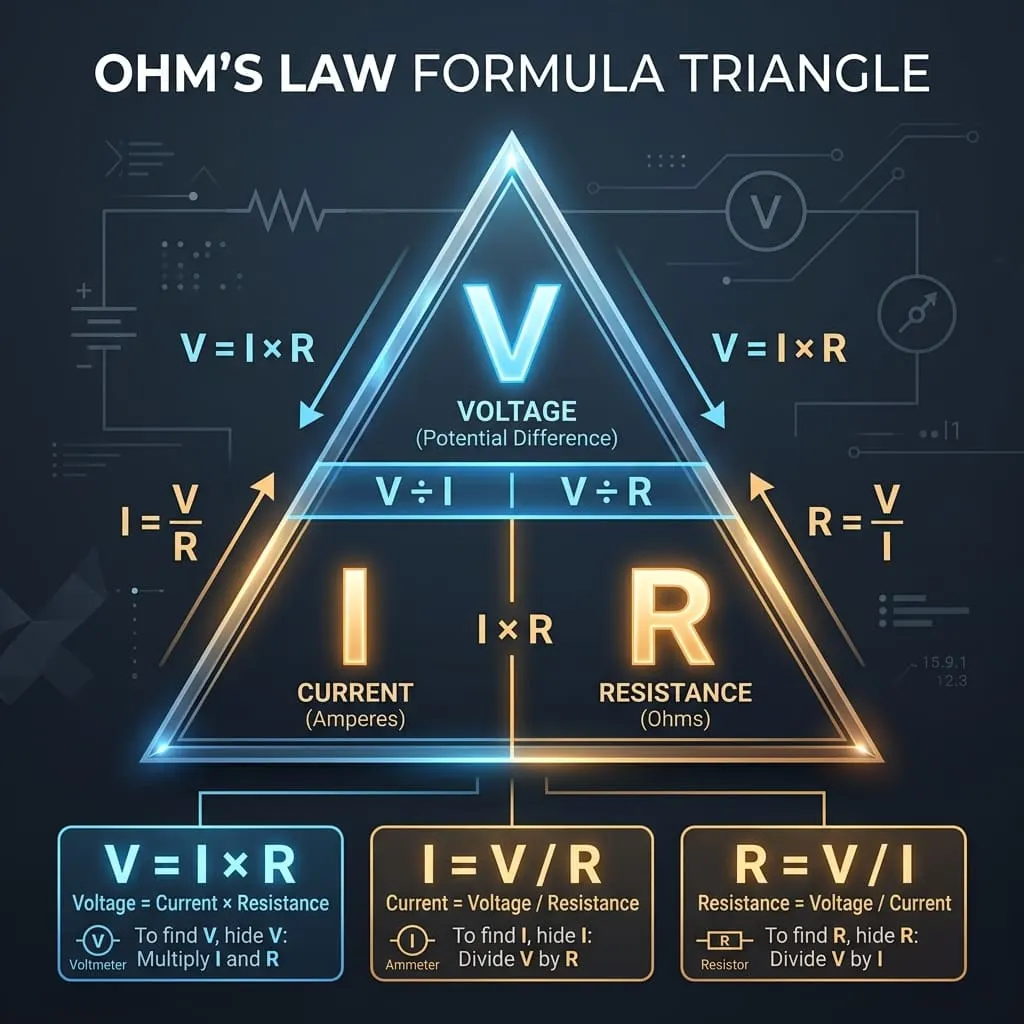
1. Introduction

From the microscopic silicon transistors pulsing billions of times every second inside modern smartphone microprocessors to high-voltage direct current (HVDC) transmission lines traversing continents, modern technological civilization operates entirely on electric charge in motion.

At the foundational bedrock of all electrical engineering, electronics, robotics, and applied physics lies a single, elegant mathematical relationship: Ohm's Law.

Formulated in 1827 by German physicist Georg Simon Ohm, this law describes the precise quantitative interrelationship among three fundamental circuit parameters: Voltage ($V$) (the electrical driving potential), Current ($I$) (the continuous flow rate of charge), and Resistance ($R$) (the intrinsic opposition to that flow).

graph LR
    V["⚡ Applied Voltage (V)
Potential in Volts (V)"] --> DIV["➗ Divided By"]
    R["🛑 Circuit Resistance (R)
Opposition in Ohms (Ω)"] --> DIV
    DIV --> I["🌊 Electric Current (I)
I = V / R in Amperes (A)"]
    I --> P["🔥 Power Dissipation (P)
P = V · I = I² · R in Watts (W)"]

Mastering Ohm's Law and its mathematical extensions allows electricians, circuit designers, and students to: - Calculate electric current draw and determine conductor gauge sizes to avoid dangerous overheating or electrical fires. - Design current-limiting bias resistors for sensitive semiconductor LEDs, microcontrollers, and sensor interfaces. - Accurately predict electrical power dissipation ($P$) and engineer thermal management systems (heat sinks, active cooling). - Troubleshoot complex direct current (DC) and alternating current (AC) power distribution networks.

2. Definitions & Analogies

2.1 The Simple Definition

In simple everyday terms: - Voltage ($V$) is the electrical "push" or pressure supplied by a power source (such as a battery or wall outlet). - Current ($I$) is the actual physical flow rate of electric charge moving through the wires and circuit components. - Resistance ($R$) is the friction or restriction that fights against that flow. - Ohm's Law states that if you increase the voltage (push), the current (flow) increases proportionally; if you increase the resistance (restriction), the current decreases proportionally.

2.2 The Formal Technical Definition

Formally, for an isotropic ohmic conductor held at a constant temperature:

"The steady electric current ($I$) flowing through a conductive medium between two terminals is directly proportional to the potential difference ($V$) across those terminals, and inversely proportional to the electrical resistance ($R$) between them."

Mathematically expressed in scalar form:

At the microscopic continuum electrodynamic level (differential field form):

Where: - $\mathbf{J}$ is the current density vector in Amperes per square meter ($\text{A/m}^2$), - $\sigma$ is the material's electrical conductivity in Siemens per meter ($\text{S/m}$), - $\rho$ is the material's electrical resistivity in Ohm-meters ($\Omega\cdot\text{m}$), - $\mathbf{E}$ is the applied electric field vector in Volts per meter ($\text{V/m}$).

2.3 The Hydraulic Water Pipe Analogy

To visualize electrical circuits intuitively, engineers frequently compare electron flow to pressurized water circulating through closed plumbing:

graph TD
    subgraph Hydraulic_Model ["💧 Hydraulic Plumbing System"]
        Pump["Elevated Water Reservoir / Pump
(Water Pressure = Voltage in Volts)"]
        Flow["Water Flow Rate (Gallons/Min)
(Volume Transport = Current in Amperes)"]
        Constriction["Narrow Pipe / Constriction Valve
(Friction Restriction = Resistance in Ohms)"]
        Pump -->|"Drives Water"| Flow
        Flow -->|"Passes Through"| Constriction
    end
    subgraph Electrical_Model ["⚡ Electrical Circuit System"]
        Battery["DC Power Supply / Battery
(Potential Difference = Voltage in Volts)"]
        Amps["Charge Transport (Coulombs/Sec)
(Electron Flow = Current in Amperes)"]
        Resistor["Circuit Load / Carbon Resistor
(Lattice Collisions = Resistance in Ohms)"]
        Battery -->|"Drives Charge"| Amps
        Amps -->|"Passes Through"| Resistor
    end

1. Voltage ($V$) $\approx$ Water Pressure: The potential energy created by a water pump or elevated water tower. Higher pressure forces more water through a pipe.
2. Current ($I$) $\approx$ Water Flow Rate: The physical volume of water passing a cross-section per second (e.g., liters per second).
3. Resistance ($R$) $\approx$ Pipe Narrowness & Obstruction: A narrow nozzle, constriction valve, or sediment buildup that restricts water flow.

3. History & Milestones in Electromagnetism

timeline
    title Milestones in Ohm's Law & Circuit Theory
    1800 : Alessandro Volta invents the Voltaic Pile (First continuous DC battery source)
    1827 : Georg Simon Ohm publishes 'Die galvanische Kette, mathematisch bearbeitet'
    1841 : The Royal Society of London awards Ohm the prestigious Copley Medal
    1845 : Gustav Kirchhoff establishes Kirchhoff's Current & Voltage Laws (KCL & KVL)
    1881 : International Congress of Electricians officially standardizes the 'Ohm' (Ω) and 'Volt' (V)
    1900 : Paul Drude formulates the classical electron collision drift model of metallic conduction

• Ohm's Experimental Breakthrough (1827): German mathematician and physicist Georg Simon Ohm set up rigorous experiments using bismuth-copper thermocouples (to eliminate the fluctuating voltage drops of early voltaic batteries) and a torsional galvanometer to measure electromagnetic deflection.
• Initial Scientific Rejection: When Ohm published his mathematical treatise Die galvanische Kette, mathematisch bearbeitet (The Galvanic Circuit Investigated Mathematically), the Prussian Minister of Education declared his theory "an incurable delusion" and forced him to resign his teaching post.
• Global Recognition & Legacy: In 1841, the British Royal Society recognized the profound truth of his empirical findings, awarding him the Copley Medal. In 1881, the International Electrical Congress formally named the international unit of electrical resistance the Ohm ($\Omega$).

4. Core Concepts & Parameters Explained

4.1 Electric Potential Difference / Voltage ($V$)

- Definition: The work required to move a unit positive charge between two distinct spatial points against an electrostatic field. - SI Unit: Volt ($\text{V}$), where $1\text{ V} = 1\text{ Joule per Coulomb } (1\text{ J/C})$. - Real-World Meaning: Voltage represents the energetic push that accelerates free conduction electrons through a metal crystal lattice.

4.2 Electric Current ($I$)

- Definition: The net rate of electric charge flow passing through a specified cross-sectional area per unit time. - SI Unit: Ampere ($\text{A}$), where $1\text{ A} = 1\text{ Coulomb per second } (6.242 \times 10^{18}\text{ electrons/s})$. - Conventional Current vs. Electron Flow: - Conventional Current: Directs from positive (+) potential to negative (-) potential (standardized in all engineering diagrams). - Electron Flow: Actual subatomic physical transport of negatively charged electrons traveling from negative (-) to positive (+) terminals.

4.3 Electrical Resistance ($R$) & Resistivity ($\rho$)

- Definition: The material property that opposes the free passage of electric current due to collisions between accelerated electrons and vibrating lattice atoms. - SI Unit: Ohm ($\Omega$), where $1\ \Omega = 1\text{ Volt per Ampere } (1\text{ V/A})$. - Pouillet's Geometric Resistance Formula: $R = \rho \frac{L}{A}$ Where $\rho$ is the material resistivity ($\Omega\cdot\text{m}$), $L$ is conductor length ($\text{m}$), and $A$ is cross-sectional area ($\text{m}^2$).

4.4 Electrical Power Dissipation & Joule Heating ($P$)

Whenever current passes through a resistive component, electrical energy converts irreversibly into thermal kinetic energy (heat). Combining Ohm's Law with Joule's First Law yields the Unified Electrical Power Equations:

• SI Unit: Watt ($\text{W}$), where $1\text{ W} = 1\text{ Joule/second } (1\text{ J/s})$.

5. The Formula Wheel & Calculation Matrix

The classic Ohm's Law and Power Wheel interlinks the four fundamental variables: Voltage ($V$), Current ($I$), Resistance ($R$), and Power ($P$).

6. Step-by-Step Computational Procedure

When solving any direct current or resistive AC circuit, follow this 4-step engineering protocol:

flowchart TD
    S1["Step 1: Identify Known & Target Parameters
(e.g., Voltage V = 120V, Resistance R = 24Ω, Solve for Current I)"] --> S2["Step 2: Normalize Values to SI Base Units
(Convert mA -> A, kΩ -> Ω, MΩ -> Ω, mV -> V)"]
    S2 --> S3["Step 3: Select the Appropriate Mathematical Equation
(I = V / R and P = V · I)"]
    S3 --> S4["Step 4: Execute Calculation & Check Thermal Limits
(Compute I, calculate Wattage P, and verify component power rating)"]

7. Comparison: Ohmic vs. Non-Ohmic Conductors

Not every electrical material or electronic device adheres to a constant linear resistance. Materials are classified into Ohmic (linear $V$-$I$ response) and Non-Ohmic (non-linear $V$-$I$ response):

graph TD
    subgraph Classification ["⚡ Electrical Conduction Behavior"]
        Ohmic["🟢 Linear Ohmic Conductors
• Pure Copper & Aluminum wire
• Precision Metal Film Resistors
• Constant-temperature Nichrome coils"]
        NonOhmic["🔴 Non-Linear Non-Ohmic Devices
• Semiconductor Diodes & LEDs (exponential threshold)
• Transistors (MOSFETs, BJTs, IGBTs)
• Incandescent Tungsten Filaments (thermal PTC)
• Gas Discharge Tubes & Arc Plasma"]
    end

8. Practical Real-World Calculation Examples

Example 1: Automotive Headlight Current Draw

- Scenario: A $12.0\text{ V}$ automotive battery powers a quartz halogen high-beam bulb with a hot filament resistance of $R = 2.40\ \Omega$. - Current Drawn: $I = \frac{V}{R} = \frac{12.0\text{ V}}{2.40\ \Omega} = \mathbf{5.00\text{ Amperes}}$

• Total Power Dissipation: $P = V \times I = 12.0\text{ V} \times 5.00\text{ A} = \mathbf{60.0\text{ Watts}}$

Example 2: Current-Limiting Resistor for an LED Circuit

- Scenario: A maker needs to power a bright blue LED ($V_{\text{forward}} = 3.20\text{ V}$, target operating current $I = 20\text{ mA} = 0.020\text{ A}$) from a $12.0\text{ V}$ DC rail. - Voltage Drop across Resistor: $V_R = V_{\text{supply}} - V_{\text{LED}} = 12.0\text{ V} - 3.20\text{ V} = 8.80\text{ V}$

• Required Resistance: $R = \frac{V_R}{I} = \frac{8.80\text{ V}}{0.020\text{ A}} = \mathbf{440\ \Omega} \quad (\text{Standard } 470\ \Omega \text{ resistor selected})$

• Resistor Power Dissipation: $P_R = I^2 R = (0.020\text{ A})^2 \times 440\ \Omega = 0.0004 \times 440 = \mathbf{0.176\text{ Watts}} \quad (176\text{ mW})$ (A standard $1/4\text{ W} = 250\text{ mW}$ resistor is adequate; a $1/2\text{ W}$ resistor provides robust thermal margin).

Example 3: Household Electric Water Heater Circuit

- Scenario: An electric water heater is rated for $4,800\text{ Watts}$ on a residential $240.0\text{ V}$ single-phase supply. - Full Load Current: $I = \frac{P}{V} = \frac{4,800\text{ W}}{240.0\text{ V}} = \mathbf{20.0\text{ Amperes}}$

• Internal Resistance of Heating Element: $R = \frac{V^2}{P} = \frac{(240.0)^2}{4,800} = \frac{57,600}{4,800} = \mathbf{12.0\ \Omega}$

Example 4: Long Distance Cable Voltage Drop

- Scenario: An outdoor irrigation pump draws $16.0\text{ A}$ over a $100\text{ meter}$ copper wire run (round trip loop resistance $R = 0.75\ \Omega$) connected to a $120.0\text{ V}$ source. - Line Voltage Drop: $V_{\text{drop}} = I \times R = 16.0\text{ A} \times 0.75\ \Omega = \mathbf{12.0\text{ Volts}}$

• Voltage Delivered to Pump: $V_{\text{load}} = 120.0\text{ V} - 12.0\text{ V} = \mathbf{108.0\text{ Volts}} \quad (10.0\%\text{ drop, exceeds } 3\%\text{ NEC guideline})$

• Thermal Cable Power Loss: $P_{\text{loss}} = I^2 R = (16.0)^2 \times 0.75 = 256 \times 0.75 = \mathbf{192.0\text{ Watts}}$

Example 5: High-Precision Shunt Resistor Voltage Sensing

- Scenario: A battery management system (BMS) measures current across a calibrated $0.005\ \Omega$ ($5\text{ m}\Omega$) precision shunt resistor. The ADC detects a voltage drop of $V = 75.0\text{ mV}$ ($0.0750\text{ V}$). - Measured Current: $I = \frac{V}{R} = \frac{0.0750\text{ V}}{0.0050\ \Omega} = \mathbf{15.00\text{ Amperes}}$

9. Real-World Engineering Case Studies

Case Study 1: Solar Photovoltaic (PV) Cable Optimization & Lifetime ROI

- Engineering Dilemma: A commercial $50\text{ kW}$ rooftop solar array operates at a nominal DC bus voltage of $600\text{ V}$, channeling $83.33\text{ A}$ through a $60\text{ meter}$ conduit run ($120\text{ m}$ round-trip total loop length). - Comparison Matrix: - Option A ($10\text{ mm}^2$ AWG #8 Copper): $R_{\text{loop}} = 0.216\ \Omega$. - Voltage Drop: $V_{\text{drop}} = 83.33\text{ A} \times 0.216\ \Omega = 18.0\text{ V}$ ($3.00\%$ loss). - Thermal Heat Loss: $P_{\text{loss}} = I^2 R = (83.33)^2 \times 0.216 = 1,500\text{ Watts} = 1.50\text{ kW}$. - Annual Energy Lost (assuming 5.0 peak sun hours/day): $1.50\text{ kW} \times 5\text{ h} \times 365\text{ days} = 2,737.5\text{ kWh/year}$. - Option B ($25\text{ mm}^2$ AWG #4 Heavy Copper): $R_{\text{loop}} = 0.0864\ \Omega$. - Voltage Drop: $V_{\text{drop}} = 83.33\text{ A} \times 0.0864\ \Omega = 7.20\text{ V}$ ($1.20\%$ loss). - Thermal Heat Loss: $P_{\text{loss}} = (83.33)^2 \times 0.0864 = 600\text{ Watts} = 0.60\text{ kW}$. - Annual Energy Lost: $0.60\text{ kW} \times 5\text{ h} \times 365\text{ days} = 1,095\text{ kWh/year}$. - Financial & Operational Payback: Upgrading to $25\text{ mm}^2$ cable saves $1,642.5\text{ kWh}$ of clean energy every year. At $\$0.16/\text{kWh}$, this generates $\$262.80/\text{year}$ in recovered revenue, paying off the heavier copper conductor cost in under 14 months while keeping wire operating temperatures far cooler.

Case Study 2: Electrical Ground Fault Current & Arc Flash Hazard

- Background: In a manufacturing plant, an ungrounded $480\text{ V}$ three-phase feeder insulation cracked, making direct contact with a grounded steel machine enclosure. - Physical Analysis: - The facility's grounding electrode system was poorly maintained, showing a high earth ground impedance of $R_{\text{ground}} = 20.0\ \Omega$. - Line-to-Ground Voltage: $V_{\text{phase}} = \frac{480\text{ V}}{\sqrt{3}} \approx 277\text{ V}$. - Resulting Ground Fault Current: $I_{\text{fault}} = \frac{277\text{ V}}{20.0\ \Omega} = \mathbf{13.85\text{ Amperes}}$

• Because the branch circuit was protected by a heavy $100\text{ A}$ thermal-magnetic circuit breaker, the $13.85\text{ A}$ fault current was completely ignored by the breaker! - The metal chassis remained energized at dangerous lethal line potential ($>200\text{ V}$), posing an extreme electrocution hazard to operators.
• Corrective Engineering Action: Electrical engineers drove chemical ground rods and bonded copper grounding grids, slashing ground impedance down to $R = 0.50\ \Omega$. Under new ground conditions: $I_{\text{fault}} = \frac{277\text{ V}}{0.50\ \Omega} = \mathbf{554\text{ Amperes}}$

This massive current instantly triggered the breaker's magnetic instantaneous trip mechanism in under $16\text{ milliseconds}$, eliminating shock and fire hazards.

10. Common Mistakes & How to Avoid Them

11. Frequently Asked Questions (FAQ)

Q1: Does Ohm's Law apply to AC (Alternating Current) circuits?

A: Yes, but resistance ($R$) is expanded to Impedance ($Z$), which accounts for frequency-dependent phase shifts from inductors and capacitors:

Q2: What happens if resistance is zero ($R = 0\ \Omega$)?

A: When resistance approaches zero, current mathematically approaches infinity ($I = V/0 \to \infty$). In physical reality, this is a short circuit. Real-world wires, switches, and batteries possess internal resistance, which limits the current to large values that can cause rapid overheating, insulation melting, sparks, or explosions unless interrupted by a fuse or breaker.

Q3: Why does a bird sitting on a high-voltage power line not get shocked?

A: The bird's two feet rest on the exact same continuous copper conductor only a few centimeters apart. The resistance of the short wire segment between its feet is minuscule ($\approx 0.0001\ \Omega$). By Ohm's Law, the voltage drop ($V = I \cdot R$) between its feet is a fraction of a millivolt. Because there is virtually zero potential difference across its body, no hazardous current flows through the high resistance of the bird.

Q4: What is the difference between Electromotive Force (EMF) and Terminal Voltage?

A: EMF ($\mathcal{E}$) is the total open-circuit potential generated by an internal chemical battery or alternator without load. Terminal Voltage ($V_{\text{term}}$) is the actual voltage available at the external terminals under load, which drops due to the battery's internal resistance ($r$):

Q5: How does human body resistance determine electrical shock severity?

A: The human body behaves like a non-linear resistor. Dry unbroken skin has a high resistance of $10,000\text{–}100,000\ \Omega$, whereas wet or punctured skin drops to $\approx 1,000\ \Omega$. At $120\text{ V}$, wet skin allows $I = 120\text{ V} / 1000\ \Omega = 120\text{ mA}$, which surpasses the threshold for ventricular fibrillation ($50\text{–}100\text{ mA}$) and is potentially fatal.

Q6: What is a shunt resistor and how does it work?

A: A shunt resistor is an ultra-low resistance, high-precision metal alloy strip (e.g., $0.001\ \Omega$) placed in series with a load. By measuring the minute millivolt drop across the known resistance, digital microcontrollers and ammeters calculate current precisely via $I = V/R$.

Q7: Why do metals have positive temperature coefficients while semiconductors have negative?

A: In metals, heating increases thermal lattice vibrations (phonons), which scatter conduction electrons and increase resistance ($\text{PTC}$). In semiconductors, heating provides thermal energy to promote valence electrons across the bandgap into the conduction band, increasing free charge carriers and decreasing resistance ($\text{NTC}$).

Q8: What is superconductivity?

A: Superconductivity is a quantum mechanical state observed in certain materials cooled below a critical transition temperature ($T_c$) where electrical resistance drops strictly to zero ($R = 0.000000\ \Omega$). In superconductors, persistent currents circulate indefinitely with zero driving voltage and zero Joule heat loss.

12. Expert Tips & Best Practices

• The 50% Power Derating Rule: Always specify resistors whose power rating is at least double ($2\times$) the anticipated steady-state dissipation ($P_{\text{rated}} \ge 2 \cdot P_{\text{actual}}$). This extends component lifespan and prevents board discoloration.
• Always Account for Wire Loop Length: When calculating voltage drop in long wire runs, remember to multiply one-way distance by $2$ to account for both the supply and return conductors.
• Use Four-Wire Kelvin Sensing for Low Resistance: When measuring resistances below $1.0\ \Omega$, standard two-lead multimeters introduce probe contact resistance errors. Always use a 4-wire Kelvin connection to measure the true voltage drop across the component.

13. Summary & Key Takeaways

• Fundamental Formula: $I = \frac{V}{R}$, $V = I \cdot R$, and $R = \frac{V}{I}$.
• Direct & Inverse Scaling: Current scales linearly with applied voltage ($I \propto V$) and inversely with circuit resistance ($I \propto 1/R$).
• Power Dissipation Coupling: Power lost to heat or mechanical work obeys $P = V \cdot I = I^2 R = \frac{V^2}{R}$ (in Watts $\text{W}$).
• Material Constraints: Strictly valid for linear ohmic conductors at constant temperature; non-linear devices (diodes, transistors) require dynamic impedance calculations.