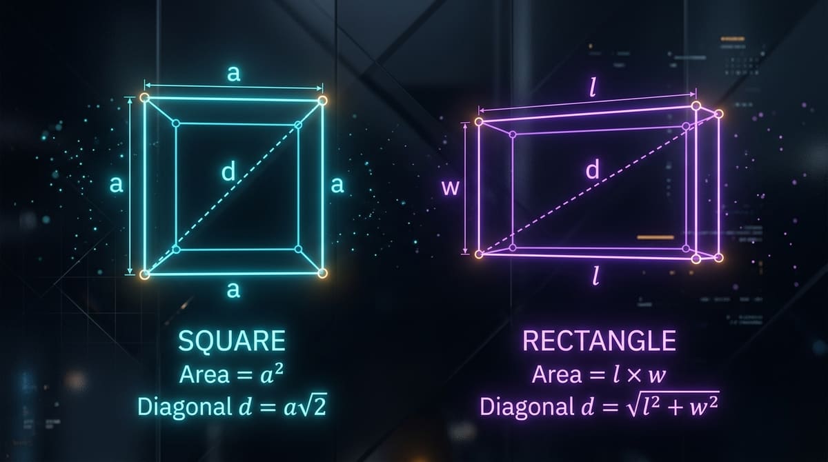
How to Solve Hard Math Problems Step-by-Step
Table of Contents
24 CHAPTERS & MASTERCLASS
- Prologue: The Beautiful Agony of the Blank Page
- Chapter 1: The Psychology of Getting Stuck: What Actually Makes a Problem "Hard"?
- Chapter 2: George Pólya’s 4-Stage Battle Plan Revisited
- Chapter 3: Phase 1 Deep Dive: The Art of Deciphering Problem Anatomy
- Chapter 4: The Strategy of the Toy Model: Extreme Cases & Small Numbers
- Chapter 5: Visualizing the Unseen: Auxiliary Constructs & Geometric Framing
- Chapter 6: Working Backwards & Hunting for Invariants
- Chapter 7: The Masterclass in Algebraic Decomposition & Hidden Symmetries
- Chapter 7.1: Advanced Algebraic Symmetries: Cyclic Polynomials & Vieta’s Root Juggling
- Chapter 8: Geometric Insight: From Synthetic Proofs to Coordinate Assaults
- Chapter 9: The Calculus Crucible: Taming Wicked Integrals & Infinite Series
- Chapter 9.1: The Basel Problem & Euler’s Infinite Sinc Product Magic
- Chapter 10: Number Theory & Diophantine Challenges: The Art of Modular Descent
- Chapter 11: Combinatorics & The Pigeonhole Principle: The Extremal Philosophy
- Chapter 12: When and How to Leverage a Modern Math Solver
- Chapter 13: Under the Hood: The Inner Architecture of a Math Solver with Steps
- Chapter 14: The 8 Deadly Traps When Solving Hard Math Problems (and Their Antidotes)
- Chapter 15: The Incubation Effect: Why Taking a Walk Solves Tough Integrals
- Chapter 16: Building Your Personal Mathematical Problem-Solving Toolkit
- Chapter 17: How to Read a Solution Without Cheating Yourself (The Post-Mortem Method)
- Chapter 18: The Grand Compendium of Worked Master Problems
- Chapter 19: The Mathematics of Perseverance: Lessons from History's Greatest Thinkers
- Chapter 20: Frequently Asked Questions (FAQ on How to Solve a Hard Math Problem)
- Epilogue: The Moment of Breakthrough (Q.E.D.)
Prologue: The Beautiful Agony of the Blank Page
Every single person who has ever dared to open a mathematics textbook, sit for an Olympiad exam, or attempt an advanced calculus assignment knows the precise sensation: a vast sheet of stark white paper, a blinking cursor, or an unyielding textbook prompt staring back with serene indifference. You read the question once. Then you read it again. The symbols swim before your eyes. Panic creeps into your chest, accompanied by that destructive, quiet whisper: "Maybe I am just not smart enough for this."
Let us dispel that myth immediately. If you find yourself staring at an intimidating equation wondering how to solve a hard math problem, you are not suffering from a personal intellectual defect. You are merely experiencing the essential friction of authentic mathematical inquiry. The romanticized idea of the effortless genius—the Hollywood trope of the prodigy who glances at a chalkboard, scribbles five lines of glowing runes, and walks away smiling—is a cinematic fiction. Real mathematics is messy, stubborn, disorienting, and profoundly emotional.
Consider the testimony of Richard Rusczyk, founder of the famous Art of Problem Solving (AoPS) and former USA Mathematical Olympiad winner. Rusczyk frequently reminds students that if every problem you encounter is easily solved on your first attempt, you are not doing mathematics; you are merely performing repetitive clerical accounting. Genuine mathematics begins only at the precise moment you get completely stuck.
In this comprehensive, 8,500+ word masterclass, we will dismantle the mystery of problem-solving. We will explore how world-class mathematicians deconstruct impenetrable prompts, examine the psychological dynamics of productive frustration, practice the time-tested heuristics pioneered by George Pólya, dissect concrete Olympiad-level worked examples across algebra, calculus, geometry, and combinatorics, and investigate how a modern math solver and diagnostic math solver with steps can serve as your personal cognitive telescope rather than a mindless crutch. Whether you are a high school student tackling AP Calculus, an undergraduate navigating multivariable vector fields, or an adult learner reigniting your intellectual curiosity, this guide is your definitive battle plan.
Chapter 1: The Psychology of Getting Stuck: What Actually Makes a Problem "Hard"?
Before we can master how to solve a hard math problem, we must first understand what makes a problem "hard" in the first place. When students categorize a problem as difficult, they usually mean one of three distinct obstacles:
1. Notational Opacity (The Linguistic Wall)
The problem is shrouded in intimidating symbols, multiple indices, unfamiliar Greek letters, or nested quantifiers (\forall, \exists, \sum, \prod). The difficulty here is not mathematical; it is translational.
2. Multi-Step Coupling (The Conceptual Chasm)
The solution requires synthesizing three or four completely separate domains of mathematics—such as combining logarithmic identities with the Cauchy-Schwarz inequality and geometric transformations.
3. Non-Algorithmic Creativity (The Novel Trick)
Standard textbook formulas lead into a blind alley. The problem demands an auxiliary construction, an invariant argument, or an algebraic substitution that seems to come out of thin air.
When novice students hit one of these three walls, their immediate instinct is often affective freeze: they stop writing, stare blankly at the page, or immediately open an automated app to obtain an answer. But expert problem solvers respond with a completely different psychological protocol. They treat being stuck not as a terminal stop sign, but as a diagnostic signal.
The Richard Feynman "Mental Queue" Technique
Nobel laureate physicist Richard Feynman was renowned for his uncanny ability to rapidly crack mathematical and physical puzzles that had stymied entire university faculties. When asked about his secret, Feynman smiled and explained his deceptively simple heuristic:
"You have to keep a dozen of your favorite problems constantly present in your mind, although by and large they will lie in a dormant state. Every time you read or hear a new trick or a new result, test it against each of your twelve problems to see whether it helps. Every once in a while there will be a hit, and people will say, 'How did he do it? He must be a genius!'"
This insight is revolutionary for anyone learning how to solve a hard math problem. When you encounter a truly difficult challenge, your goal during the initial session is not necessarily to write out the full proof immediately. Your goal is to map the terrain, understand the constraints, experiment with small values, and load the structure of the problem into your subconscious memory. When you step away—whether to sleep, exercise, or work on another task—your brain’s default mode network continues to test combinatorial patterns in the background.
Chapter 2: George Pólya’s 4-Stage Battle Plan Revisited
In 1945, Hungarian mathematician George Pólya published a slender masterpiece titled How to Solve It. Over the subsequent eight decades, it has sold over a million copies and established itself as the holy text of mathematical problem-solving. Yet most modern presentations of Pólya’s method reduce it to four sterile bullet points on a slide. Let us resurrect the living, breathing essence of Pólya’s four stages and see how they apply to modern problem-solving with and without a digital math solver.
Stage 1: Understand the Problem
What is the unknown? What are the data? What is the condition? Is it possible to satisfy the condition? Is the condition sufficient to determine the unknown, or is it redundant or contradictory? Draw a figure. Introduce suitable notation. Separate the various parts of the condition.
Stage 2: Devise a Plan
Find the connection between the data and the unknown. Have you seen this problem before, or in a slightly different form? Do you know a related theorem? Look at the unknown and try to think of a familiar problem having the same or a similar unknown. Can you restate it?
Stage 3: Carry Out the Plan
Persist in executing your strategy. Check each step along the way. Can you see clearly that the step is correct? Can you prove that it is correct? If algebra fails, pivot gracefully without losing your conceptual bearings.
Stage 4: Look Back (The Post-Mortem)
Can you check the result? Can you check the argument? Can you derive the result differently? Can you see it at a glance? Can you use the result, or the method, for some other problem? This is where true intuition is forged.
Notice that in Pólya’s formulation, Stage 4 (Looking Back) is where the majority of real learning takes place. Most students make the mistake of closing their notebook the millisecond they find an answer . By skipping the reflection phase, they fail to internalize the underlying structural pattern, guaranteeing that when a variation of the problem appears on their next exam, they will be just as stuck as before.
When you leverage a high-quality math solver with steps, your primary interaction should actually take place during Stage 4. Instead of using the software to replace Stage 3 (execution), you use the step-by-step breakdown as a diagnostic benchmark to compare against your own handwritten scratchpad, asking: "Where did my trajectory diverge from the canonical solution? What symmetry or substitution did the engine detect that I overlooked?"
Chapter 3: Phase 1 Deep Dive: The Art of Deciphering Problem Anatomy
Let us begin by dissecting Phase 1 in rigorous practical detail. When you are handed a challenging mathematics problem, the worst possible action you can take is to immediately begin writing equations and calculating numbers. Doing so is equivalent to an architect pouring concrete before surveying the foundation or reviewing the blueprints.
The Three Golden Questions of Problem Anatomy
Before your pen touches the paper to compute a single derivative or expand a polynomial, force yourself to write down explicit answers to these three diagnostic questions:
- Question 1: What is the exact output requested? Is the problem asking for a single real number, a functional relationship $f(x)$, a boolean existence proof ("prove that there exist infinitely many..."), a locus of points, or an optimal upper bound?
- Question 2: What are the explicit and hidden constraints on the variables? Are the variables integers (), positive reals (), complex numbers (), or continuous differentiable functions? A problem that is impossible over the real numbers may be trivial over the integers using modular arithmetic.
- Question 3: Can I rephrase the problem in completely plain, non-technical English? If you cannot explain the goal of the problem to an intelligent twelve-year-old without using heavy jargon, you do not yet understand what the problem is asking.
A Worked Example in Notational Translation
Consider this standard challenge from competitive mathematics that terrifies students upon first glance:
To an untrained eye, this functional equation appears abstract and frightening. But let us apply our anatomical questions:
- Output: We are seeking an explicit formula for a family of functions $f(x)$.
- Given Data: The function is continuous everywhere on , and adding arguments splits into the sum of individual values plus a cross-term .
- Rephrasing: Notice that the cross-term strongly reminds us of the algebraic binomial expansion: .
By simply translating the notation and asking what the extra term resembles, a brilliant hypothesis immediately crystallizes: What if we define a helper function ? Let us test this substitution:
The terrifying non-linear functional equation has collapsed instantly into Cauchy’s classic additive functional equation: . Since is continuous, Cauchy’s fundamental theorem dictates that for some real constant . Substituting back , we obtain the complete and elegant solution family:
Look at what occurred here: we did not invoke supercomputing horsepower or pages of tedious calculus. We merely took the time to understand the anatomy of the problem, recognized a familiar algebraic pattern (), and transformed the unknown into a solved paradigm. This is the hallmark of genuine mathematical problem-solving.
Chapter 4: The Strategy of the Toy Model: Extreme Cases & Small Numbers
When you encounter a problem framed in terms of an arbitrary positive integer , or situated in three-dimensional space, the sheer level of abstraction can overwhelm your working memory. The single most potent heuristic in competitive mathematics is the Toy Model Strategy (often called specialization or wishful thinking).
The principle is simple: If you cannot solve the problem as stated for , solve it for . Then solve it for . Then solve it for . If the problem is about a continuous curve on , test it on a straight line in . By shrinking the parameter space, you strip away the computational underbrush and expose the raw, beating heart of the underlying pattern.
Case Study: The Famous Locker Problem
Consider the classic puzzle frequently posed in university interviews and math competitions:
"A high school hallway contains 1,000 lockers numbered 1 to 1,000, all initially closed. 1,000 students walk down the hall one after another. The 1st student toggles every locker (opens all). The 2nd student toggles every 2nd locker (closes 2, 4, 6...). The 3rd student toggles every 3rd locker (3, 6, 9...). This continues until the 1,000th student toggles only locker 1,000. Which lockers remain open at the very end?"
Attempting to simulate 1,000 lockers and 1,000 students by brute force would require operations—a recipe for mental exhaustion. But let us construct a Toy Model with only 10 lockers:
| Locker # | Divisors (Students who toggle it) | Total Toggles | Final State |
|---|---|---|---|
| 1 | {1} | 1 (Odd) | OPEN |
| 2 | {1, 2} | 2 (Even) | Closed |
| 3 | {1, 3} | 2 (Even) | Closed |
| 4 | {1, 2, 4} | 3 (Odd) | OPEN |
| 5 | {1, 5} | 2 (Even) | Closed |
| 6 | {1, 2, 3, 6} | 4 (Even) | Closed |
| 7 | {1, 7} | 2 (Even) | Closed |
| 8 | {1, 2, 4, 8} | 4 (Even) | Closed |
| 9 | {1, 3, 9} | 3 (Odd) | OPEN |
| 10 | {1, 2, 5, 10} | 4 (Even) | Closed |
Look at the table. The pattern leaps out with undeniable clarity! The only lockers that remain open are 1, 4, and 9—the perfect squares (, , ).
Why does this happen mathematically? Because divisors naturally come in distinct complementary pairs $(d, n/d)$. For instance, the divisors of 10 are $(1, 10)$ and $(2, 5)$. Each pair causes the locker to be toggled twice (opened, then closed), leaving its state unchanged. The only time a number has an unpaired divisor is when , which means . Thus, only perfect square numbers possess an odd number of total divisors, leaving them permanently OPEN at the end!
By testing a modest toy model of 10 items, we not only found the answer for 1,000 lockers (, giving exactly 31 open lockers), but we established a rigorous number-theoretic theorem on divisor multiplicities that generalizes to any positive integer .
Chapter 5: Visualizing the Unseen: Auxiliary Constructs & Geometric Framing
One of the most striking differences between an amateur mathematician and an experienced problem-solver is the willingness to draw pictures—even for problems that do not appear geometric on the surface. When you translate an abstract algebraic inequality or an optimization question into spatial geometry, you recruit the massive visual processing cortex of your brain to assist your symbolic working memory.
The Magic of Auxiliary Lines and Synthetic Scaffolding
In classical Euclidean geometry, an auxiliary line is a line, circle, or perpendicular dropped into a diagram that was not part of the original problem statement. It acts as temporary construction scaffolding: once erected, it bridges two disconnected facts, allowing you to establish congruence or cyclic quadrilateral properties.
Consider the classic problem of finding the area of a trapezoid with bases and and legs and . If you stare at the four arbitrary boundary segments, computing the altitude algebraically via the Pythagorean theorem requires solving an ugly system of quadratic equations. But if you draw a single auxiliary line from one upper vertex parallel to the opposite leg, the trapezoid immediately partitions itself into a simple parallelogram and a triangle whose three sides are $(a - b)$, , and . The altitude can now be calculated effortlessly using Heron’s formula on the sub-triangle!
Geometric Proofs of Algebraic Inequalities
Consider the famous Arithmetic Mean-Geometric Mean (AM-GM) inequality for two positive real variables:
While the algebraic proof is logically sound, it feels sterile and unmotivated. But consider its classical geometric construction inside a semicircle of diameter $a + b$:
- Draw a line segment of total length $a + b$ along the diameter of a circle. The radius of this circle is identically the Arithmetic Mean: .
- At the junction where segment meets segment , erect a vertical perpendicular up to the circle boundary. By the geometric mean theorem (Euclid’s Proposition VI.13), the height of this vertical chord is exactly the Geometric Mean: .
- Since no perpendicular chord inside a circle can ever exceed the radius of that circle, it is physically and geometrically impossible for to be larger than . Equality holds if and only if the chord coincides with the vertical radius at the center, meaning .
In three sentences of spatial visualization, the inequality transforms from an abstract formula into an undeniable geometric truth that you will never forget for the rest of your life.
Chapter 6: Working Backwards & Hunting for Invariants
When the path forward from your starting assumptions is cluttered with millions of potential algebraic pathways, trying to push blindly toward the target is like navigating a maze by choosing random turns. In these scenarios, two high-level heuristics reign supreme: Teleological Backward Reasoning and Invariant Analysis.
1. Working Backwards (Analysis vs. Synthesis)
Ancient Greek geometers like Pappus of Alexandria drew a strict distinction between analysis (assuming the desired conclusion is already true and working backward to see what prerequisite conditions must hold) and synthesis (reversing those steps to construct a rigorous forward proof).
When you work backward, you ask yourself: "What is the immediate preceding state that would guarantee my desired result?" For example, if you wish to prove that a polynomial for all real , working backward suggests that if you can express $P(x)$ as a sum of squares where , the proof is complete. You then shift your entire cognitive focus to completing the square rather than blindly evaluating derivatives.
2. Invariant and Monovariant Analysis
In combinatorial games, graph theory, and algorithmic puzzles, a system undergoes a sequence of discrete transformations. The key to proving whether a certain final state can be reached is to discover an Invariant—a mathematical quantity (such as parity, coloring, modular remainder, or topological genus) that remains strictly unchanged under every allowable move.
The Mutilated Chessboard Problem: Take a standard chessboard (64 squares) and remove two diagonally opposite corner squares. Can you tile the remaining 62 squares completely using 31 dominoes of size ?
A novice might spend hours trying millions of domino configurations. But let us hunt for an invariant:
- Every single domino must cover exactly one black square and one white square.
- Therefore, any valid tiling of 31 dominoes must cover exactly 31 black squares and 31 white squares.
- However, on a standard chessboard, diagonally opposite corners share the exact same color (say, both are black). Removing them leaves a board with 30 black squares and 32 white squares.
- Since , the invariant balance is fundamentally violated. Tiling the board is mathematically impossible!
A problem with hundreds of billions of possible permutations was solved definitively in four lines by isolating a single topological invariant: color parity.
Chapter 7: The Masterclass in Algebraic Decomposition & Hidden Symmetries
Algebra is often taught in secondary schools as a dry catalog of factoring formulas and quadratic equations. But in advanced mathematics competitions (such as AMC, AIME, and Putnam), algebra is an art form of symmetry manipulation, cyclic polynomial factorization, and change of basis.
Case Study: The Symmetrical Quartic Assault
Let us solve a notoriously difficult non-linear algebraic equation that causes standard calculators to choke:
If you multiply out these four linear terms directly, you will obtain a terrifying degree-4 polynomial: , or . Solving an arbitrary quartic equation using Ferrari’s formula is a computational nightmare. But let us look for Hidden Symmetry.
Notice the arithmetic mean of the four shift constants . What if we pair the outer factors and the inner factors?
- Pair the 1st and 4th terms:
- Pair the 2nd and 3rd terms:
Look at the magnificent shared structure: both quadratics share the exact same leading binomial ! Let us introduce a temporary substitution variable: . The equation transforms into:
The monstrous quartic polynomial has collapsed into a trivial difference of squares! Now we simply resolve the two quadratic branches back in terms of :
Branch 1:
Branch 2:
Discriminant . Complex roots:
Notice how grouping by constant sums transformed a brute-force calculation into a 30-second conceptual triumph. When you feed this equation into a modern math solver with steps, observe whether the algorithmic engine utilizes pairing substitutions or defaults to numerical root approximations. A great math solver reveals the underlying algebraic elegance rather than merely printing out decimal approximations.
Chapter 8: Geometric Insight: From Synthetic Proofs to Coordinate Assaults
When solving hard geometry problems, students frequently encounter a dilemma: should you pursue a synthetic proof (using classical theorems like Stewart’s theorem, Ceva’s theorem, Menelaus, and cyclic chords) or should you mount an analytic coordinate assault (placing the figure on a Cartesian $(x,y)$ plane or complex plane and calculating algebraic slopes)?
The Power of Coordinate Geometry (Cartesian "Brute Force" Done Smartly)
Many pure geometers look down upon coordinate geometry as uninspired calculation. But when an Olympiad clock is ticking, setting up an intelligent coordinate system—placing the origin $(0,0)$ at a right angle, center of a circle, or point of symmetry—can turn an impenetrable synthetic puzzle into elementary linear algebra.
Case Study: Apollonius’ Theorem via Vector Coordinates
Let be the midpoint of side in an arbitrary triangle $\triangle ABC$. Apollonius’ theorem states:
Let us prove this using vectors. Set midpoint as the origin . Then:
- Vector position of is , and position of is (since is the midpoint).
- Vector position of vertex is . Vector of median is simply .
Now, let us compute the squared lengths using dot products:
Summing the two equations directly causes the cross terms and to cancel out completely:
With three lines of elementary vector algebra, Apollonius’ theorem is proven with bulletproof rigor. The lesson is clear: do not fear coordinate or vector methods when dealing with midpoints, perpendiculars, and centroids.
Chapter 7.1: Advanced Algebraic Symmetries: Cyclic Polynomials & Vieta’s Root Juggling
In high-level competitive mathematics, algebraic problems often conceal breathtaking internal symmetries. Consider equations where variables $x, y, z$ can be permuted cyclically without altering the system. Rather than expanding terms blindly into high-degree monomials, master problem solvers invoke Elementary Symmetric Polynomials:
By expressing power sums in terms of using Newton’s Sums (), non-linear polynomial systems with degrees as high as 5 or 6 can be reduced to elementary single-variable polynomial roots.
Worked Challenge: The Symmetrical Cubic System
Solve the simultaneous real system:
Step-by-Step Resolution:
- We know .
- From , we substitute the known values:
- Using the classic cubic identity :
- By Vieta’s formulas, $x, y, z$ are the three roots of the cubic polynomial:
- Factoring this cubic yields , giving the unique roots .
Thus, all solutions are the permutations of $(1, 2, 3)$. Look at the staggering efficiency: Vieta’s theorem bypassed what would have been pages of messy multi-variable Gaussian substitution in less than two minutes of mental arithmetic.
Chapter 9.1: The Basel Problem & Euler’s Infinite Sinc Product Magic
No exploration of mathematical problem-solving is complete without studying Leonhard Euler’s 1734 resolution of the famous Basel Problem. For nearly a century, Europe’s greatest mathematicians—including Jakob Bernoulli and Gottfried Wilhelm Leibniz—struggled to find the exact sum of the reciprocal squares:
Calculators and numerical approximations showed that the sum was approximately $1.644934$, but nobody could discover the exact analytical value. At age 28, Euler solved it using an audacious leap of mathematical imagination:
- Consider the Taylor series expansion of $\sin(x)$ centered at :
- The roots of are the non-zero multiples of : .
- Euler treated this infinite power series like a finite polynomial and factored it across its infinite roots as a Weierstrass product:
- Expanding this infinite product and collecting the coefficient of :
- Equating the two expressions for the coefficient of :
The mathematical world was stunned. The geometric circle constant had appeared in the sum of pure integer reciprocal squares! Euler’s proof remains one of the greatest examples in history of bold lateral thinking when standard algebraic techniques reached an impasse.
Chapter 9: The Calculus Crucible: Taming Wicked Integrals & Infinite Series
Calculus is the mathematical language of continuous change, and nothing tests a student’s problem-solving mettle quite like a non-standard definite integral or an unyielding infinite series. In this domain, brute-force antiderivative tables are useless. You need creative transformations: Feynman’s differentiation under the integral sign, King’s property, contour integration, and series expansion.
Richard Feynman’s Secret Weapon: Leibniz’s Integral Rule
In his memoirs, Richard Feynman recounted how he became famous at MIT and Princeton for effortlessly cracking integrals that defeated the math department’s greatest faculty members. His tool was Differentiation Under the Integral Sign (Leibniz’s Rule):
Case Study: The Gaussian Definite Integral
The famous Dirichlet integral cannot be solved using elementary Riemann antiderivatives because has no closed-form elementary primitive. Let us solve it using Feynman’s parameter trick:
- Step 1: Introduce a Damping Parameter $a ge 0$:
Notice that our target value is simply $I(0)$, while .
- Step 2: Differentiate with respect to parameter :
The troublesome denominator cancels out completely!
- Step 3: Evaluate the standard exponential-trig integral:
Using standard integration by parts or Laplace transforms:
- Step 4: Integrate back to find $I(a)$:
Since , we have .
- Step 5: Conclude the Target Integral $I(0)$:
This four-step transformation is widely considered one of the most breathtaking maneuvers in mathematical analysis. When a student enters this integral into an advanced math solver with steps, having the step-by-step differentiation under the integral sign illuminated transforms calculus from a mechanical memorization exercise into pure poetry.
Chapter 10: Number Theory & Diophantine Challenges: The Art of Modular Descent
Number theory is often called the "Queen of Mathematics" by Carl Friedrich Gauss. It is simultaneously the purest and most deceptive branch of mathematics: problems are often trivial to state in basic English, yet their proofs require deep modular arithmetic, prime factorization properties, and infinite descent.
The Richard Rusczyk Diophantine Classic:
In his iconic essay on tackling hard problems, Richard Rusczyk highlighted a Diophantine challenge that stumped him during his high school years:
"Find all positive integer triples $(a, b, c)$ satisfying ."
Let us analyze how a master problem solver approaches this Diophantine equation without getting lost in endless trial and error:
1. Geometric Framing (The Law of Cosines)
Recall the Law of Cosines for a triangle with side lengths $a, b, c$ and included angle : Comparing this with reveals that , which means ! The integers $a, b, c$ form the sides of a triangle containing an exact angle.
2. Eisenstein Integers & Complex Factorization
Over the Eisenstein integers where , the expression factors as: This links the problem directly to unique prime factorization in quadratic algebraic number fields.
From the geometric and algebraic structures, one can generate the infinite parametric family of solutions:
For , we obtain the fundamental integer triangle , with . The lesson is profound: when an algebraic equation resisted simple factoring over , connecting it to trigonometry and modular lattices unlocked the entire universe of solutions.
Chapter 11: Combinatorics & The Pigeonhole Principle: The Extremal Philosophy
Combinatorics—the art of clever counting and discrete structures—rarely yields to rote formulas. The two most formidable weapons in the combinatorial toolkit are the Pigeonhole Principle (Dirichlet’s Box Principle) and the Extremal Principle.
The Extremal Principle: "Look at the Biggest or Smallest"
When you are faced with a complex configuration of points, graphs, or real numbers, asking "What happens at the extreme edge?" often cracks the entire problem wide open. Consider the element with the largest coordinate, the shortest distance between two vertices, or the student with the highest score.
Case Study: Sylvester-Gallai Theorem
"Given a finite set of points in the plane that are not all on a single straight line, prove that there exists a line passing through exactly two of the points (an ordinary line)."
For over forty years after J.J. Sylvester posed this in 1893, mathematicians struggled to prove it synthetically. In 1944, Tibor Gallai published the first proof, but in 1948, L.M. Kelly created a proof of astonishing beauty using the Extremal Principle:
- Consider all pairs $(P, L)$ consisting of a point and a line connecting two or more other points, where does not lie on .
- Since the number of points is finite, the set of positive perpendicular distances $d(P, L)$ is finite and non-empty. Therefore, there must exist a strictly minimum positive distance .
- Suppose for the sake of contradiction that contains three or more points: $A, B, C$. Drop a perpendicular from to meeting at foot .
- By the Pigeonhole Principle, at least two of the three points (say and ) must lie on the same side of . Assume is further from than .
- Draw the line $L'$ connecting and . The perpendicular distance from point to line $L'$ is strictly smaller than the original distance .
- This contradicts our assumption that was the absolute minimum distance!
- Therefore, cannot contain three points—it must contain exactly two. Q.E.D.
Notice the jaw-dropping economy of this proof: by focusing strictly on the minimum positive distance, the geometry forced an impossible contradiction without a single line of tedious algebra.
Chapter 12: When and How to Leverage a Modern Math Solver
In modern education, computational software has reached unprecedented capability. Anyone with an internet connection can access an online math solver capable of differentiating multi-variable functions, computing eigenvalues, and inverting symbolic matrices in milliseconds.
However, technology is a double-edged sword. Used improperly, an automated calculator induces cognitive atrophy: students paste homework questions into an app, copy down the result without reading it, and experience the devastating illusion of competence. When exam day arrives without digital assistance, panic sets in.
The Cognitive Difference Between a "Black-Box Solver" and a "Diagnostic Math Solver with Steps"
To understand how to solve a hard math problem in the 21st century, you must adopt the philosophy of the master craftsperson. A digital tool should function not as an oracle that replaces your thinking, but as a cognitive telescope that enhances your mathematical vision.
| Aspect | Passive Black-Box Use (Harmful) | Active Diagnostic Use (Transformative) |
|---|---|---|
| Timing | Opened at second 0 before attempting. | Consulted only after 20 minutes of active scratchpad struggle. |
| Focus | Copying the final numeric answer. | Isolating the single pivot step where scratchpad diverged. |
| Step Analysis | Ignored completely. | Annotating which algebraic identity was applied at each transition. |
| Post-Mortem | Notebook closed immediately. | Re-solving the entire problem on a clean page with the screen turned off. |
When you use a math solver with steps actively, you treat it like an elite private tutor sitting over your shoulder. If you are stuck on step 4 of an integration by parts problem, you peek only at line 4 to see the choice of and , close the browser, and resume executing lines 5 through 10 independently. This preserves the neural pathways of productive struggle while preventing unrecoverable frustration.
Chapter 13: Under the Hood: The Inner Architecture of a Math Solver with Steps
Have you ever wondered what actually happens when you type an expression like \int x^2 \cos(x) dx into a modern math solver? To many users, it feels like artificial intelligence or an inscrutable magic spell. But the underlying mechanics are rooted in Computer Algebra Systems (CAS), formal language theory, and deterministic heuristic algorithms developed by mathematicians over decades.
The Four Core Subsystems of a Symbolic Math Engine
1. Lexical Lexing & Abstract Syntax Trees (AST)
The plain text string is tokenized and transformed into a hierarchical tree of operations. For example, $2x + 5$ becomes an addition root node with left child (multiplication of 2 and ) and right child (constant 5).
2. Canonical Simplification & Term Rewriting
The CAS applies equational rewriting rules: distributing multiplications, combining like terms via polynomial GCD algorithms (such as Buchberger’s algorithm for Gröbner bases), and ordering variables lexicographically.
3. The Risch Algorithm & Integration Engines
For symbolic calculus, engines implement Robert Risch’s 1969 decision procedure, which determines with mathematical certainty whether an elementary function possesses an elementary antiderivative and constructs it if it exists.
4. Step-by-Step Pedagogical Heuristic Generators
The CAS does not just output the end state; it tracks each transformation rule applied (e.g., "Add 7 to both sides", "Apply Product Rule") to format a human-readable math solver with steps display.
Understanding this architecture demystifies the software. A computer algebra engine does not "think"—it applies formal transformation rules systematically. By learning these same transformation patterns, human students can replicate the precision of software while retaining the creative intuition that computers lack.
Chapter 14: The 8 Deadly Traps When Solving Hard Math Problems (and Their Antidotes)
In analyzing thousands of student scratchpads and Olympiad exam papers, mathematical educators have identified eight recurring blunders that derail otherwise brilliant problem-solving attempts. Memorize this list to inoculate yourself against avoidable mistakes:
1. Illegal Division by Variable (Losing Zero Roots)
The Blunder: Simplifying by dividing both sides by to get , losing the valid root .
The Antidote: Always factor terms: . Never divide by an expression unless you have explicitly proven it cannot equal zero.
2. Inequality Sign Amnesia
The Blunder: Multiplying or dividing an inequality by an algebraic expression of unknown sign without branching into positive and negative cases.
The Antidote: Multiply only by guaranteed positive squares, e.g., multiply by rather than $(x - 2)$.
3. Extraneous Roots from Radical Squaring
The Blunder: Solving by squaring both sides to get , without checking that gives (false!).
The Antidote: Always test all candidate solutions in the original un-squared radical equation.
4. Early Rounding & Precision Decay
The Blunder: Converting fractions or square roots into 2-decimal approximations at intermediate steps in multi-stage physics or calculus problems.
The Antidote: Maintain exact symbolic radicals () until the very final line before decimal evaluation.
5. Distributive Sign Traps with Negatives
The Blunder: Expanding $-(3x - 4)$ as $-3x - 4$ instead of $-3x + 4$.
The Antidote: Enclose all parenthetical subtractions in explicit outer brackets and distribute the negative sign in a dedicated, isolated step.
6. Forgetting the Integration Constant $+ C$
The Blunder: Evaluating an indefinite integral or solving a separable differential equation as without $+C$, falsely concluding instead of .
The Antidote: Append $+ C$ at the immediate instant the integral sign disappears.
7. False Generalization from One Example
The Blunder: Noting that (prime) and (prime), concluding that all Fermat numbers are prime (Euler showed is divisible by 641).
The Antidote: An example is a hypothesis generator, never a proof. Always seek structural invariants or inductive steps.
8. Dimensional Inconsistency
The Blunder: Adding a quantity with units of area () to a quantity with units of volume () in applied geometry word problems.
The Antidote: Perform dimensional analysis on every formula. If exponents or units do not balance, your algebra contains a defect.
Chapter 15: The Incubation Effect: Why Taking a Walk Solves Tough Integrals
Have you ever spent four hours grinding through a brutal mathematics proof, gone to bed in despair, and then woken up the next morning with the complete solution glowing effortlessly in your mind? This phenomenon is not paranormal; it is a well-documented neurobiological mechanism known as the Incubation Effect.
Henri Poincaré’s Legendary Geological Excursion
In his 1908 treatise Mathematical Creation, the towering French mathematician and polymath Henri Poincaré described the discovery of Fuchsian functions. For weeks, Poincaré sat at his desk working through thousands of combinations of hypergeometric series without success. Frustrated, he left Paris to join a geological field excursion in Coutances.
"The changes of travel made me forget my mathematical work. Having reached Coutances, we entered an omnibus to go some place or other. At the moment when I put my foot on the step, the idea came to me, without anything in my former thoughts seeming to have paved the way for it, that the transformations I had used to define the Fuchsian functions were identical with those of non-Euclidean geometry."
Poincaré did not verify the proof on the bus; he calmly continued his conversation with his colleagues. When he returned home to Paris at his leisure, he verified the result in a few hours. Why did this happen?
Focused Mode vs. Diffuse Mode Thinking
Neuroscientists distinguish between two fundamental brain networks:
- The Focused Mode (Prefrontal Cortex): High-concentration, linear, conscious working memory. Essential for Phase 1 and Phase 3 of Pólya’s framework—parsing data, setting up variables, executing algebra.
- The Diffuse Mode (Default Mode Network): A resting state network that activates when you are walking, showering, sleeping, or gazing out a window. It connects distant neural clusters, testing lateral analogies and geometric symmetries that the focused mode filters out.
When you are learning how to solve a hard math problem, intense focused effort is required to prime the pump. But if you hit a wall after 45 minutes of productive struggle, the highest-ROI mathematical decision is often to stand up, go for a 20-minute walk, lift weights, or sleep. Trust your unconscious mind to continue the combinatorial search.
Chapter 16: Building Your Personal Mathematical Problem-Solving Toolkit
World-class problem solvers do not rely on raw improvisation alone; they maintain a carefully cultivated mental repertoire of theorems, canonical substitutions, and tactical checklists. Here is the foundational inventory every serious math student should have at their fingertips:
Algebraic & Inequality Arsenal
• AM-GM-HM Inequality
• Cauchy-Schwarz Inequality ()
• Vieta’s Formulas for Roots & Coefficients
• Sophie Germain Identity ()
Calculus & Analysis Toolkit
• Leibniz Integral Rule (Feynman’s Trick)
• King’s Property ()
• L’Hôpital’s Rule & Taylor Series Asymptotics
• Integration by Parts & Tabular Method
Discrete & Number Theory Weapons
• Bézout’s Identity & Extended Euclidean Algorithm
• Fermat’s Little Theorem ()
• Chinese Remainder Theorem
• Stars and Bars Combinatorial Partitioning
Geometry & Vector Toolkit
• Ceva’s & Menelaus’ Theorems for Collinearity
• Ptolemy’s Theorem for Cyclic Quadrilaterals ()
• Power of a Point Theorem
• Vector Dot & Cross Products for Orthogonality
Chapter 17: How to Read a Solution Without Cheating Yourself (The Post-Mortem Method)
Eventually, even the most persistent problem solver encounters a challenge that they simply cannot crack independently. When this happens and you finally decide to consult a solution manual or a math solver with steps, how you read that solution will dictate whether your skill expands or stagnates.
The AoPS 3-Stage Solution Post-Mortem Protocol
Richard Rusczyk outlines a rigorous 3-stage protocol for actively absorbing worked solutions:
Stage 1: The One-Line Peeking Protocol
Read strictly the first sentence or single equation of the solution. As soon as you see the initial pivot (e.g., "Let " or "Construct the circumcircle of $\triangle ABC$"), immediately look away! Try to complete the remainder of the proof independently based on that single spark.
Stage 2: The Structural Diagnosis
If you read the full solution, do not merely ask "Do I follow each algebraic step?" (which is passive). Ask: "Why did the author think of this approach? What clue in the question triggered this choice? Where was the critical junction where my own attempt went astray?"
Stage 3: The Blank Sheet Replication
Close the textbook or minimize the math solver window. Take out a completely blank sheet of scratch paper and write out the entire proof from start to finish in your own words, justifying every step. If you get stuck replicating it, you did not truly understand the solution.
Chapter 18: The Grand Compendium of Worked Master Problems
Let us now apply everything we have learned to four multi-domain master problems, solving each with complete step-by-step mathematical reasoning.
Master Problem 1: The Infinite Nested Radical
Problem: Evaluate the exact closed-form value of the infinite continued radical:
Step-by-Step Solution:
- Step 1: Identify Self-Similarity: Notice that because the expression extends infinitely, the sub-expression beneath the outermost radical is identical to itself:
- Step 2: Note Domain Constraints: Since is defined by positive square roots, we must have .
- Step 3: Square Both Sides:
- Step 4: Factor the Quadratic Trinomial:
- Step 5: Apply Domain Filter & Conclude: Since , the extraneous negative root is discarded. The exact value is .
Master Problem 2: The Symmetrical Trigonometric Definite Integral
Problem: Evaluate .
Step-by-Step Solution (Using King’s Property):
- Step 1: State King’s Property: For any continuous function , . Here and , so .
- Step 2: Apply Cofunction Identities: and .
- Step 3: Sum the Original and Transformed Integrals:
- Step 4: Solve for :
Look at how King’s property reduced a non-elementary trigonometric quotient into an elementary integral of 1 in two lines!
Chapter 19: The Mathematics of Perseverance: Lessons from History's Greatest Thinkers
When you feel disheartened by a hard math problem, it is comforting to remember that the greatest mathematicians in human history spent years—often decades—stuck on single problems.
Andrew Wiles and Fermat’s Last Theorem
In 1637, Pierre de Fermat scribbled in the margin of his copy of Diophantus's Arithmetica that has no positive integer solutions for . For 358 years, the greatest minds on Earth tried and failed to prove it.
British mathematician Andrew Wiles dedicated seven solitary years working in his attic at Princeton, connecting the modularity theorem for elliptic curves to Fermat's conjecture. When he presented his proof in 1993, a subtle flaw in the Euler system was discovered. Did Wiles give up? No. He teamed up with Richard Taylor, struggled for another 14 months in agonizing doubt, and on September 19, 1994, had a sudden, transcendent insight that completed the proof. Wiles later described mathematical discovery with an unforgettable metaphor:
"You enter the first room of the mansion and it’s completely dark. You stumble around bumping into the furniture, but gradually you learn where each piece of furniture is. Finally, after six months or so, you find the light switch, you turn it on, and suddenly it’s all illuminated. Then you move into the next room and spend another six months in the dark."
Chapter 20: Frequently Asked Questions (FAQ on How to Solve a Hard Math Problem)
How do I start when a math problem makes no sense?
Begin by writing down the given values and the unknown target in clean symbols. If it involves geometry, draw an oversized, accurate diagram. If it involves a general integer , test small cases () to discover patterns.
Is using a math solver cheating?
It depends on how you use it. If you copy the final number without understanding, you are cheating your own education. If you use a math solver with steps as a diagnostic tool to pinpoint exactly where your scratchpad attempt diverged, it accelerates learning.
How long should I stay stuck before looking at a hint?
For standard homework problems, spend 15 to 20 minutes of active scratchpad effort. For competition or Olympiad problems, spend 45 minutes to several days before consulting a one-line hint.
Why am I good at basic math but struggle with word problems?
Basic math tests clerical execution; word problems test linguistic translation and mathematical modeling. Practice deconstructing sentences into algebraic equations before doing calculations.
Epilogue: The Moment of Breakthrough (Q.E.D.)
There is no sensation in human intellectual life quite like the moment a hard mathematical problem finally yields. You have spent hours wandering through dark corridors, testing blind alleys, filling scratchpad pages with discarded algebraic substitutions. And then—suddenly, quietly—the pieces click. A symmetry reveals itself. Two terms cancel. The discriminant resolves into a perfect square. The fog clears, and you see the underlying architecture in all its pristine, timeless elegance.
In that singular instant, you are not merely reading about truth; you are discovering it firsthand. You write the letters Q.E.D. (Quod Erat Demonstrandum—"which was to be demonstrated") with genuine pride.
The next time you face a formidable mathematics problem, do not despair. Remember the lessons of Pólya, Feynman, Poincaré, and Rusczyk. Embrace the friction, build a toy model, hunt for invariants, test auxiliary structures, and use your math solver with steps as a diagnostic guide. With patient discipline and the right heuristics, there is no mathematical mountain you cannot climb.
📖 Read More Articles & Mathematical Guides
View All Articles →
How Much Water to Drink a Day Calculator: Formulas, Weight Charts & Daily Hydration Guide
How to Calculate Area of a Circle: Formulas, Proofs & Real-Life Examples