How to Find the Greatest Common Factor (GCF): The Definitive Guide
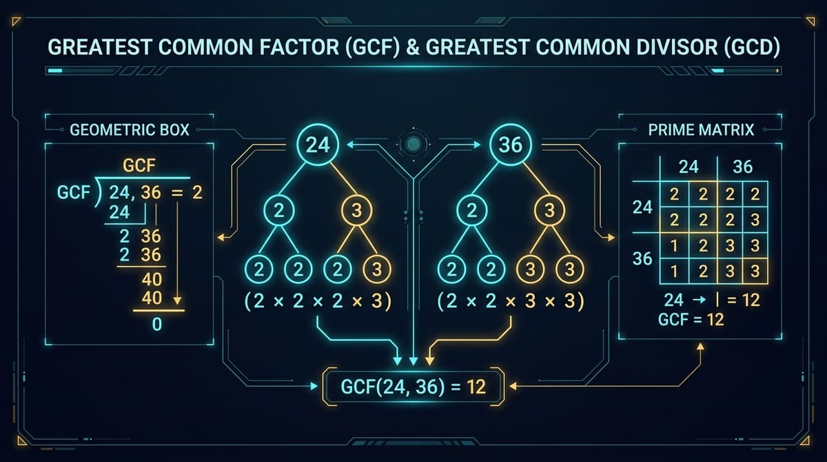
Table of Contents
15 CHAPTERS & ALGORITHMIC PROOFS
- 1. The Architectural Core of Divisibility & The Definition of GCF
- 2. Method I: The Factor Listing & Set Intersection Method
- 3. Method II: Prime Factorization & The Minimum Exponent Rule
- 4. Method III: The Repeated Division (Ladder / Cake) Method
- 5. Method IV: Euclid's 2,300-Year-Old Algorithm (The Granddaddy of Algorithms)
- 6. Method V: The Euclidean Subtraction (Antyphairesis) Method
- 7. Method VI: The Extended Euclidean Algorithm & Bézout's Identity
- 8. Method VII: Stein's Binary GCD Algorithm (The Modern CPU Workhorse)
- 9. The Golden Link: GCF and LCM Dual Identity & Multi-Variable Proofs
- 10. Generalizing to Multiple Numbers: Associative Reduction of gcd(a, b, c, d)
- 11. Algebraic Factoring: Finding the GCF of Monomials and Polynomials
- 12. Real-World Applications: RSA Cryptography, Signal Processing & Mechanics
- 13. Computational Complexity: Gabriel Lamé's Theorem & Fibonacci Worst Cases
- 14. Algorithm Comparison & Decision Matrix
- 15. Frequently Asked Questions (FAQ)
1. The Architectural Core of Divisibility & The Definition of GCF
In the monumental history of computer science and pure mathematics, few ideas possess the enduring elegance and universal utility of the Greatest Common Factor (GCF). In his seminal multi-volume treatise The Art of Computer Programming, renowned computer scientist Donald Knuth famously celebrated Euclid’s method for calculating the greatest common divisor as "the granddaddy of all algorithms, because it is the oldest nontrivial algorithm that has survived to the present day."
First formalized around 300 BC in Book VII of Euclid's Elements, the greatest common factor transcends basic arithmetic. Today, the exact same mathematical principles power modern RSA public-key internet encryption, synchronize digital audio digital-to-analog converters (DACs), optimize mechanical gear tooth wear, simplify complex algebraic rational fractions, and resolve high-dimensional linear Diophantine equations in discrete engineering.
💡 Direct Answer & Formal Mathematical Definition
The Greatest Common Factor (GCF)—also interchangeably termed the Greatest Common Divisor (GCD), Highest Common Factor (HCF), or Greatest Common Measure (GCM)—of two or more non-zero integers and is the largest positive integer that divides both and without leaving a remainder.
Where the notation $d \mid a$ reads " divides evenly" (meaning there exists an integer such that ).
Universal Axiomatic Properties of Divisors
To master the computation of common factors, one must first recognize the fundamental structural properties governing integers under divisibility:
- Identity with 1: For any positive integer , . The number 1 is the universal trivial factor of every integer.
- Identity with Self: For any integer , . Every number is its own largest divisor.
- Identity with Zero: For any non-zero integer , . Because zero divided by any non-zero number is zero (), every non-zero number divides zero; hence, the largest shared divisor between and is $|a|$.
- The Undefined Zero-Zero Case: $\gcd(0, 0)$ is mathematically undefined (or conventionally set to 0 in computational number theory libraries), because every integer in divides 0, making the set of common divisors infinite with no upper bound.
- Sign Invariance: . Divisors are symmetrically signed, but the GCF is conventionally defined as strictly positive ().
- Commutativity & Associativity: and .
- Distributive Law over Multiplication: For any positive integer , .
GCF & GCD Method Selection Decision Matrix
Select the optimal mathematical algorithm based on input magnitude, computation environment, and algebraic context.
Factor Listing & Set Intersection
Systematically list all divisor pairs $(d, n/d)$ up to and extract the maximal common intersection element.
Prime Factorization / Ladder
Decompose integers into prime powers and apply minimum exponents: .
Euclidean Modulo Algorithm
Repeated division remainder steps: . Solves large numbers in milliseconds.
Euclidean Subtraction
Original geometric subtraction (anthyphairesis): without needing division.
Extended Euclidean (Bézout)
Calculates linear integer coefficients $x, y$ satisfying for modular inverse calculation.
Stein's Binary GCD Algorithm
Replaces division with binary bit-shifts (>> 1) and parity tests, maximizing low-level CPU efficiency.
2. Method I: The Factor Listing & Set Intersection Method
The most intuitive way to discover the greatest common factor is the Factor Listing (Set Intersection) Method. In this approach, we systematically generate all positive divisors of each number, represent them as mathematical sets, and find the maximum element in their set intersection.
How to Systematically Find All Factors Without Missing Any
A frequent student mistake when listing factors is guessing randomly. To list factors with 100% mathematical certainty, always test candidate divisors in ascending order from up to . Whenever divides without a remainder, it instantly yields a conjugate factor pair:
Worked Example: Find the GCF of 72 and 108 using Factor Listing
Step 1: Determine all factors of 72:
We test divisors up to :
- $5 \nmid 72$
- $7 \nmid 72$
Step 2: Determine all factors of 108:
We test divisors up to :
Step 3: Construct the Set Intersection :
While factor listing is outstanding for teaching early school arithmetic, its computational complexity is . For numbers with 10 or more digits, listing all divisors requires billions of division checks. For massive 500-digit integers, listing factors would take trillions of years—even if every supercomputer on Earth worked in parallel.
3. Method II: Prime Factorization & The Minimum Exponent Rule
By invoking the Fundamental Theorem of Arithmetic, every positive integer can be expressed uniquely as a product of prime powers:
The Formal Minimum Exponent Theorem
Let and be two positive integers decomposed over the complete set of distinct prime bases :
Then, the Greatest Common Divisor is rigorously given by the product of every prime raised to the minimum exponent occurring in both factorizations:
Worked Example: Find the GCF of 360 and 840 using Prime Factorization
Step 1: Decompose 360 into prime factors:
Step 2: Decompose 840 into prime factors:
Step 3: Construct the Prime Comparison Table:
| Prime Factor () | Power in 360 () | Power in 840 () | GCF Component | |
|---|---|---|---|---|
| 2 | 3 | 3 | ||
| 3 | 2 | 1 | ||
| 5 | 1 | 1 | ||
| 7 | 0 | 1 |
Step 4: Multiply the Minimum Exponent Powers:
4. Method III: The Repeated Division (Ladder / Upside-Down Cake) Method
The Repeated Division Ladder Method (frequently referred to as the Upside-Down Division Cake or Grid Method) is a compact, highly reliable paper-and-pencil technique. It extracts shared prime factors simultaneously across all input numbers without requiring complete, separate factor trees.
Step-by-Step Algorithmic Procedure:
- Write the target numbers horizontally on a single line separated by commas.
- Identify any common prime number that divides all numbers evenly. Place this prime to the left of the vertical bar.
- Divide each number by this common divisor and write the resulting quotients directly underneath.
- Repeat this process on the new row of quotients until the numbers share no common divisor greater than 1 (i.e., until they become mutually coprime).
- Calculate GCF: Multiply all the prime divisors along the left vertical column.
- Bonus LCM Calculation: Multiply all numbers along the left column and across the bottom row in an "L-shape".
Worked Example: Find the GCF and LCM of 48, 72, and 120
  2 |  48 ,   72 ,  120
----+-------------------
  2 |  24 ,   36 ,   60
----+-------------------
  2 |  12 ,   18 ,   30
----+-------------------
  3 |   6 ,    9 ,   15
----+-------------------
        2 ,    3 ,    5   (Stop: 2, 3, 5 share no common factor)
1. Calculating GCF (Left Column Product):
2. Calculating LCM (Full 'L' Shape Product):
5. Method IV: Euclid's 2,300-Year-Old Algorithm (The Granddaddy of Algorithms)
When dealing with large numbers—such as 6-digit accounting values or 2,048-bit cryptographic primes—listing factors or finding prime factorizations becomes mathematically infeasible. Euclid's Algorithm solves the GCF problem in milliseconds without factoring a single number.
The Fundamental Division Invariant Theorem
By the Euclidean Division Lemma, for any two integers and with , there exist unique integers (quotient) and (remainder) such that:
The Invariant Rule: Any integer that divides both and must also divide their remainder . Conversely, any divisor that divides both and must also divide . Therefore:
By repeatedly replacing $(a, b)$ with , the numbers shrink exponentially at every cycle until the remainder reaches . The last non-zero remainder is the exact Greatest Common Divisor!
Worked Benchmark: Find the GCF of 12,378 and 3,054 using Euclid's Algorithm
| Step () | Division Equation () | Quotient () | Remainder () |
|---|---|---|---|
| 1 | 4 | 162 | |
| 2 | 18 | 138 | |
| 3 | 1 | 24 | |
| 4 | 5 | 18 | |
| 5 | 1 | 6 (Last Non-Zero) | |
| 6 | 3 | 0 (Termination) |
Geometric Proof by Rectangle Tiling
In ancient Greece, numbers were understood as geometric lengths. To find $\gcd(a, b)$ geometrically, imagine a floor of dimensions . The Greatest Common Divisor represents the largest possible square tile that completely covers the entire floor without cutting or overlapping.
If we lay down maximal squares of size , we fit complete squares, leaving an uncovered strip of dimensions . Any square that tiles the entire rectangle must also tile this remaining strip. Repeating this procedure leads directly to the final square tile of side length $\gcd(a, b)$.
6. Method V: The Euclidean Subtraction (Antyphairesis) Method
Prior to the widespread adoption of algebraic division, Euclid formulated his algorithm via repeated geometric subtraction, known in ancient Greek as Antyphairesis (mutual subtraction).
The underlying mathematical property states:
Worked Example: Find the GCF of 105 and 42 via Subtraction
Note on performance: If $a \gg b$ (e.g., and ), subtraction requires $500,000$ operations, whereas division modulo solves it in 1 step. Subtraction is preserved primarily for educational clarity and specialized hardware lacking division units.
7. Method VI: The Extended Euclidean Algorithm & Bézout's Identity
One of the most profound theorems in modern number theory is Bézout's Identity (named after Étienne Bézout, 1730–1783). It proves that the greatest common divisor of any two integers can always be expressed as their integer linear combination:
The integers and are called the Bézout coefficients. The Extended Euclidean Algorithm computes $\gcd(a, b)$ while simultaneously finding and through backward substitution.
Why Bézout's Identity Is Critical: Modular Inverses in RSA Cryptography
In modern cybersecurity, to decrypt an RSA message, the computer must compute the modular multiplicative inverse . This is equivalent to solving the linear Diophantine equation:
Worked Example: Solve and find
Forward Pass (Standard Euclidean Division):
Backward Substitution Pass:
Start with the equation expressing remainder 1:
Substitute :
Substitute :
Bézout coefficients: , .
To find the positive modular inverse: .
Check: !
8. Method VII: Stein's Binary GCD Algorithm (The Modern CPU Workhorse)
Published by Josef Stein in 1967, the Binary GCD Algorithm replaces expensive division and modulo operations with ultra-fast hardware bitwise operations: bit-shifts (division by 2, u >> 1), bitwise AND parity checks (u & 1), and subtractions.
The 4 Binary Reduction Rules:
- Rule 1 (Both Even): If and are both even, .
- Rule 2 (One Even, One Odd): If is even and is odd, . (The factor 2 cannot be common).
- Rule 3 (Both Odd): If and are both odd and , . (The difference of two odd numbers is always even, permitting an instant bitshift).
- Rule 4 (Base Case): and .
High-Performance JavaScript / C Implementation
function binaryGCD(u, v) {
  if (u === 0) return v;
  if (v === 0) return u;

  // Find common power of 2 using trailing zeros
  let shift = 0;
  while (((u | v) & 1) === 0) {
    u >>= 1;
    v >>= 1;
    shift++;
  }

  // Remove remaining factors of 2 from u
  while ((u & 1) === 0) u >>= 1;

  while (v !== 0) {
    // Remove factors of 2 from v
    while ((v & 1) === 0) v >>= 1;

    // Now u and v are both odd. Subtract smaller from larger
    if (u > v) {
      const temp = u;
      u = v;
      v = temp;
    }
    v = v - u;
  }

  // Restore common factors of 2
  return u << shift;
}
9. The Golden Link: GCF and LCM Dual Identity & Multi-Variable Proofs
Between the Greatest Common Factor and the Least Common Multiple (LCM) lies one of the most celebrated dualities in algebra:
Rigorous Number-Theoretic Proof:
Express and as prime power products: and .
By definition:
Multiplying both expressions yields:
For any real numbers , the algebraic identity holds unconditionally. Therefore:
A dangerous misconception is assuming . This is false!
Counterexample: For : and . Their product is .
The correct three-variable formula is governed by the Inclusion-Exclusion Principle:
10. Generalizing to Multiple Numbers: Associative Reduction of gcd(a, b, c, d)
Because the GCD operator is strictly associative and commutative, finding the greatest common factor of an arbitrary list of integers is achieved by cascading pairwise GCDs:
Worked Example: Find the GCF of 180, 270, 450, and 540
11. Algebraic Factoring: Finding the GCF of Monomials and Polynomials
In high school and collegiate algebra, finding the Greatest Common Factor is the mandatory first step before factoring quadratic equations, trinomials, or simplifying rational algebraic fractions.
Rules for Finding the GCF of Algebraic Monomials:
- Find the numerical GCF of all coefficients.
- For each shared variable, take the lowest exponent appearing across all terms.
- Multiply the numerical GCF by the variable components.
Worked Algebraic Factoring Examples
Example A: Find the GCF of and
- Numerical GCF:
- Variable :
- Variable :
- Variable :
- Monomial GCF:
Example B: Factor the Polynomial
1. Find GCF of terms: , lowest variable power is .
2. Divide each term by to construct factored polynomial:
12. Real-World Applications: RSA Cryptography, Signal Processing & Mechanics
🔐 1. RSA Internet Encryption
Every HTTPS secure session requires generating public/private keypairs. The public exponent (commonly 65537) must satisfy . The private key is computed via the Extended Euclidean Algorithm to solve .
⚙️ 2. Mechanical Gear Trains
In high-performance automotive transmissions and industrial turbines, engineers design gear tooth counts and to be coprime (, known as the hunting tooth design). This ensures every tooth contacts every opposing tooth uniformly, eliminating repetitive harmonic wear.
🎵 3. Digital Audio Sample Rates
When converting standard CD audio (44.1 kHz) to studio film audio (48.0 kHz), DSP chips compute . Audio stream decimation interpolates the signal by upsampling by and downsampling by .
📦 4. Logistics & Architectural Tiling
Packaging engineers calculate GCF to pack dissimilar inventory items into identical shipping boxes with zero wasted volume, and civil architects use GCF to determine maximum square paving slabs without cutting tiles on site.
13. Computational Complexity: Gabriel Lamé's Theorem & Fibonacci Worst Cases
How fast is Euclid's algorithm? In 1844, French mathematician Gabriel Lamé published a historic proof in the Comptes Rendus establishing one of the earliest results in computational complexity theory:
📜 Gabriel Lamé's Theorem (1844)
The number of division steps required by the Euclidean Algorithm to find $\gcd(a, b)$ with is never greater than 5 times the number of decimal digits in the smaller number .
The Absolute Worst-Case Input: Consecutive Fibonacci Numbers
Lamé proved that the slowest possible input for Euclid's algorithm occurs when and are two consecutive Fibonacci numbers: and .
Because , every quotient in the Euclidean chain is exactly , which represents the slowest possible remainder reduction:
Even in this theoretical worst case, the algorithm terminates in logarithmic time , making it exponentially faster than trial factorization .
14. Algorithm Comparison & Decision Matrix
Use the following technical comparison matrix to select the ideal Greatest Common Factor algorithm for your computational constraints:
| Algorithm | Time Complexity | Space | Optimal Input Size | Primary Advantage |
|---|---|---|---|---|
| I. Factor Listing | Visual clarity for early education. | |||
| II. Prime Factorization | Reveals fundamental prime structure. | |||
| III. Division Ladder | Simultaneously finds GCF and LCM on paper. | |||
| IV. Euclidean Division | Any magnitude () | Universal standard; zero factoring required. | ||
| V. Euclidean Subtraction | Similar magnitude | Requires only subtraction, no division units. | ||
| VI. Extended Euclidean | Cryptographic integers | Computes Bézout $x, y$ & modular inverses. | ||
| VII. Stein's Binary GCD | bitwise | Hardware & CPUs | Up to 30% faster on modern CPU registers. |
15. Frequently Asked Questions (FAQ)
What is the difference between GCF, GCD, HCF, and GCM?
There is no mathematical difference. They are regional naming conventions for the exact same concept:
• GCF (Greatest Common Factor): Standard term in United States elementary and middle school curriculum.
• GCD (Greatest Common Divisor): Standard term in university number theory, computer science, and algebra worldwide.
• HCF (Highest Common Factor): Standard term in the United Kingdom, India, Singapore, Australia, and Commonwealth curricula.
• GCM (Greatest Common Measure): Historical term used by Euclid and 19th-century mathematicians.
Can the GCF of two numbers be equal to 1?
Yes! When , the numbers and are called relatively prime or coprime. They share no common factors other than 1. For example, 8 and 15 share no prime factors (), so , even though neither 8 nor 15 is a prime number.
How do you find the GCF of negative numbers?
Take the absolute values of the numbers: . By mathematical convention, the GCF is always defined as a positive integer (). For example, .
What is the GCF of 0 and any integer n?
For any non-zero integer , . This is because every non-zero integer divides 0 (), so the largest divisor shared between and 0 is $|n|$ itself. However, $\gcd(0, 0)$ is undefined because every positive integer divides 0, meaning there is no greatest element.
Can you find the GCF of fractions?
Yes! For two simplified fractions and , the greatest common divisor fraction is given by the formula: For example: .
Why is the GCF always less than or equal to the smaller number?
A factor of a positive integer cannot be strictly greater than (since for any , which is not an integer). Because the common factor must divide both and , it must satisfy and , which guarantees .
📖 Read More Articles & Mathematical Guides
View All Articles →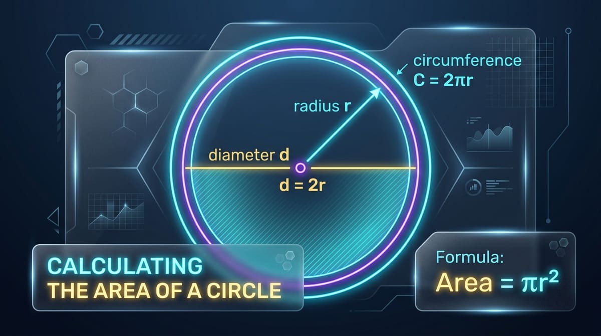
How to Calculate Area of a Circle: Formulas, Proofs & Real-Life Examples
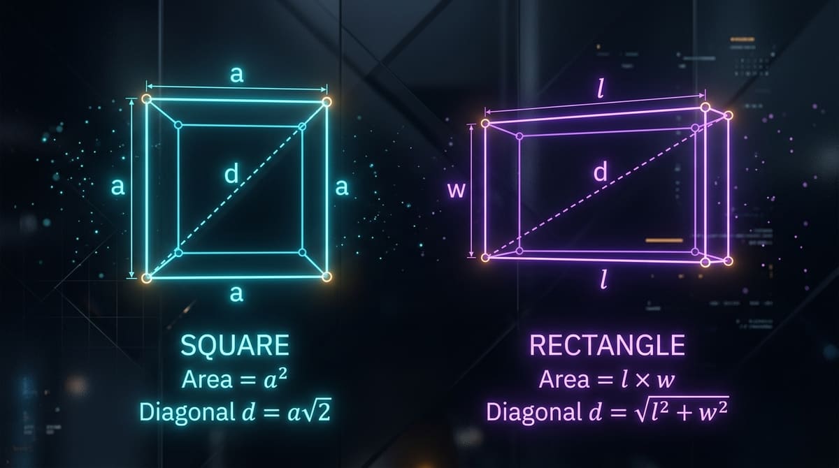
How to Calculate Area of Square and Rectangle: Complete Formulas, Diagonals & Real-Life Examples